- Research article
- Open access
- Published:
A review of some geometric integrators
Advanced Modeling and Simulation in Engineering Sciences volume 5, Article number: 16 (2018)
Abstract
Some of the most important geometric integrators for both ordinary and partial differential equations are reviewed and illustrated with examples in mechanics. The class of Hamiltonian differential systems is recalled and its symplectic structure is highlighted. The associated natural geometric integrators, known as symplectic integrators, are then presented. In particular, their ability to numerically reproduce first integrals with a bounded error over a long time interval is shown. The extension to partial differential Hamiltonian systems and to multisymplectic integrators is presented afterwards. Next, the class of Lagrangian systems is described. It is highlighted that the variational structure carries both the dynamics (Euler–Lagrange equations) and the conservation laws (Nœther’s theorem). Integrators preserving the variational structure are constructed by mimicking the calculus of variation at the discrete level. We show that this approach leads to numerical schemes which preserve exactly the energy of the system. After that, the Lie group of local symmetries of partial differential equations is recalled. A construction of Lie-symmetry-preserving numerical scheme is then exposed. This is done via the moving frame method. Applications to Burgers equation are shown. The last part is devoted to the Discrete Exterior Calculus, which is a structure-preserving integrator based on differential geometry and exterior calculus. The efficiency of the approach is demonstrated on fluid flow problems with a passive scalar advection.
Introduction
With the increasing performance of computers (speed, parallel processing, storage capacity, ...), one might think that it is not worth to design completely new algorithms to solve numerically basic problems in mechanics. It is tempting to think that to simulate physics with a fair precision, one just has to take small enough time and space steps. Yet, experiments show that, even with an academic problem such as an harmonic oscillator, classical numerical schemes which rely on a direct discretization of the equations are unable to predict correctly the solution over a long time period, even with a fine time and space grids. In fact, the equation of a system may hide physically very important properties, such as conservation laws, which are destroyed by these schemes, leading to a meaningless prediction or a blow up.
Many physical properties of a system are encoded within a geometric structure of the equation. A natural way to correctly predict these properties is then to preserve exactly the geometric structure during the simulation. This is the foundation principle of geometric integrators. This approach of discretization generally enables a better representation of the physics of the system and a particular robustness for a long time or/and large space simulation.
The aim of this article is to draw the attention of computational mechanics specialists to geometric integrators. However, since many geometric structures, and consequently many geometric integrators, exist, it is not conceivable to describe all of them. Instead, we will focus on the most widely used. The main properties of these integrators will be listed. Examples of construction will be presented and illustration on mechanical systems will be given. Many references will be provided throughout the article for each part of the article for more complete details.
One of the oldest geometric structures used in physics is the symplecticity of Hamiltonian systems. When it can be written in a symplectic framework, an ordinary differential equation (ODE) exhibits a preservation of a differential form, the symplectic form, over time. The symplectic formulation also permits to obtain conservation laws via Nœther’s theorem [1,2,3]. Symplectic integrators are built to preserve the symplecticity of the flow at the discrete level. One of the first works on symplectic integrators is that of Vogeleare in 1956 (see [4]), followed by many papers and books in the 1980’s [5,6,7,8,9,10,11]. Since then, an abundant literature can be found on the subject.
Many symplectic systems come from a variational problem. In this case, the equation represents a trajectory which minimizes a Lagrangian action. A way of building a symplectic integrator for such a problem is to discretize the Lagrangian function and solve the corresponding discrete variational problem. This approach yields variational integrators [4, 12,13,14]. Variational integrators are automatically symplectic and momentum preserving. They have been developed since the 1960’s in optimal control theory and the 1970’s in mechanics ([15,16,17,18,19,20,21,22], see [13] for a more complete historical overview). Note that variational integrators can be extended to solve efficiently non-variational problems by embeeding the latter into a larger Lagrangian system [23, 24].
Attempts on the extension of the symplectic geometry to fields appeared from the 1950’s with the works of Gallisot [25] and Dedecker (see [26,27,28]), followed by many others a decade later [28,29,30,31]. That gave rise to two major theories. The first one is based on the polysymplectic approach in which the symplectic form is extended into a vector-valued form [32,33,34,35,36,37]. The other theory led to the multisymplectic notion where the cotangent bundle is replaced by the bundle of k-forms [26, 30, 38, 39]. Nœther’s theorem has been extended to the polysymplectic and multisymplectic approaches [40,41,42,43]. At the computational side, the extension of symplectic integrators to partial differential equations (PDEs) led to multisymplectic integrators [44,45,46,47,48,49]. They have been used to solve a wide range of problems in physics [16, 50,51,52,53].
Other equations of mechanics cannot straightforwardly formulated with a Lagrangian functional nor a (multi-)symplectic structure. It is the case of many mechanical dissipative systems. Yet, many of them have important invariance properties, called symmetries [54], under some transformations. Symmetries play a fundamental role since they may encode exact model solutions (self-similar, vortex, shock solutions, ...), conservation laws via Nother’s theorem or physical principles (Galilean invariance, scale invariance, ...) [55,56,57,58,59,60,61,62,63,64,65,66,67,68]. They have also been used for modelling purposes such as the establishment of wall laws in turbulent flows or the development of turbulence models [69,70,71,72,73,74,75,76]. It is then important that numerical schemes do not break symmetries if one wishes to reproduce numerically the cited model solutions and properties. Preserving the symmetries of the equations at the discrete level is the founding key of invariant integrators [77,78,79,80,81,82,83], as will be seen in “Invariant integrators” section. Note that the symmetry structure does not exclude simplecticity structure. So, combining symplectic/variational algorithm and invariant scheme is feasible, but not done in this article.
Recently, a new generation of geometric integrators, called discrete exterior calculus (DEC), has been developed. It appeared from the observation that equations of physics, especially electromagnetism, are better written with differential forms (instead of vector fields) and exterior calculus operators (see [84,85,86,87] and the series of papers of Bossavit [88,89,90,91,92]). DEC aims at developing a discrete version of the theory of exterior calculus, and more generally differential geometry, where most equations of physics are formulated. This framework offers naturally coherent discretization of derivation operators (divergence, gradient, curl) since, in exterior calculus, they are represented by a single operator \({\text {d}}\), the exterior derivative. The basic tools in DEC theory are discrete differential forms, seen as simplicial cochains. This approach of discrete form could be found in the work of Tonti [93] (see also [94]) in the 1970’s, and later in [95,96,97,98]. The current development of DEC has been inspired by the works of Bossavit in electromagnetism [99,100,101,102,103,104,105]. More recent works in electromagnetism include [106,107,108,109]. In the field of mechanics, DEC has been employed to solve Darcy, Euler and Navier–Stokes equations in some basic configurations [110,111,112], to geometrizes elasticity problems [113, 114] or to solve port-Hamiltonian systems [115]. DEC belongs to the family of cochain-based mimetic discretization methods described in [116]. Among the members of this family, we can cite the covolume method [117], spline-based cochain discretization [118], mimetic spectral elements [119,120,121] or spectral DEC [122, 123]. Other compatible discretization techniques include the Finite Element Exterior Calculus (FEEC) [124,125,126], mimetic finite differences ([127] and references therein) and works in [128,129,130,131,132].
In the next section, we recall the basic principle of symplectic geometry. We then show why and how to build symplectic and multisymplectic integrators. In “Variational integrators” section, variational systems and variational integrators are presented. A total variation approach, which extends the usual presentation of Lagrangian mechanics, is used. Indeed, with a total variation consideration, an energy equation (and momentum equation in case of PDE) naturally arises. This equation can be used to build, for instance, energy-preserving schemes. Invariant integrators are dealt with in “Invariant integrators” section. The approach used is that of Kim [79, 133] and Chhay and Hamdouni [80] which consists in modifying classical schemes to make them invariant. At last, discrete exterior calculus is described in “Discrete exterior calculus” section. Simulations of fluid flows convecting a passive scalar are presented.
Some theoretical tools of differential geometry are used in this article to highlight the geometry structures. Their definition can be found, for example, in [1, 54, 134,135,136,137,138,139,140,141,142,143]. However, their use has been limited (at the risk of using formal definitions) and the examples are simple enough for readers more interested in the computational aspect.
Symplectic integrators
We begin with a brief introduction to Hamiltonian mechanics. Interested readers can find deeper presentations in [1, 2, 144,145,146].
Hamiltonian system and flow
Hamiltonian system
Let \((\mathcal S,\omega )\) be a symplectic manifold, consisting of a smooth manifold \(\mathcal S\), the phase manifold, equiped with a symplectic structure, i.e. a closed and non-degenerate two-form field \(\omega \). Let H be a Hamiltonian function on \(\mathcal S\), that is a smooth function \(H:\mathcal S\rightarrow \mathbb {R}\). The Hamiltonian function H determines a unique vector field \({\mathbf {X}}_H\) defined by:

the symbol  standing for the interior productFootnote 1 and \({\text {d}}H\) is the differential or exterior derivative of H. A Hamiltonian system on \((\mathcal S,\omega )\), associated to the Hamiltonian function H, is a dynamical system \(\mathbf {s}(t)\) governed by the equation
Let \({\Phi }_t\) be the Hamiltonian flow, i.e. the map
which, to any initial condition \(\mathbf {s}_0\), associates the solution at time \(t\ge 0\). The Hamiltonian flow \({\Phi }_t\) is a symplectomorphism, meaning that along trajectories,
where \({\Phi }_t^*\) is the pull-backFootnote 2 of \({\Phi }_t\). In other words, the Hamiltonian flow preserves the symplectic structure of the equation.
The symplectic manifold \(\mathcal S\) has necessarily an even dimension, say \(2n_{\mathbf q}\), and there exists canonical coordinates \(\mathbf {s}=(\mathbf q,\mathbf p)^{\mathsf {T}}\) belonging to an open set of \(\mathbb {R}^{n_{\mathbf q}}\times {\mathbb {R}}^{n_{\mathbf q}}\) in which Eqs. (1) and (2) can be written as follows:
the Hamiltonian H being a function \((t,\mathbf q,\mathbf p)\in {\mathbb {R}}\times \mathbb {R}^{n_{\mathbf q}}\times {\mathbb {R}}^{n_{\mathbf q}}\mapsto H(t,\mathbf q,\mathbf p)\in \mathbb {R}\). Equation (5) can be written in a more compact way as follows:
where \(\nabla H=(\nabla _{\mathbf q}H,\nabla _{\mathbf p}H)^{\mathsf {T}}\) and \(\mathbb J\) is the skew-symmetric matrix
\(I_{n_{\mathbf q}}\) being the identity matrix of \({\mathbb {R}}^{n_{\mathbf q}}\). The matrix \(\mathbb J\) is the matricial representation of the symplectic form \(\omega \). In canonical coordinates, \(\omega \) writes:
where \(\wedge \) is the exterior product symbol.Footnote 3
In canonical coordinates, the symplecticity property (4) reduces to
in matricial form, and to
in exterior calculus notation.
Flow of a numerical scheme
The flow of a numerical integration scheme of Eq. (2) is defined as
where \(\mathbf {s}^n\) is the numerical approximation, at a discrete time \(t=t^n\), of the solution \(\mathbf {s}(t)\) corresponding to an initial condition \(\mathbf {s}^0\). A numerical integrator is said symplectic if, like the exact flow, it preserves the symplectic structure of the equation. More rigorously, a numerical scheme is symplectic if its flow verifies
The numerical pull-back \({\Phi }_n^*\) is an approximation of the exact pull-back \({\Phi }^*_t\) at \(t=t^n\).
In practice, we only consider one-step incremental integrators. For such integrators, it is more convenient to work with the one-step flow
instead of \({\Phi }_n\). Note that \({\Phi }_{{\Delta }t}\) may depend on n. As examples, the flow of the explicit Euler integration scheme of (2) is
The flow of a second order Runge–Kutta scheme is
where
And the flow of a fourth order Runge–Kutta scheme is
where
A sufficient condition for a one-step incremental integrator to be symplectic is that \({\Phi }_{{\Delta }t}\) is symplectic (for any n), that is:
In matricial and in exterior calculus forms in canonical coordinates, this condition writes:
and
Failure of classical integrators
In this section, we show, through elementary examples, that the use of non-structure-preserving algorithms may have dramatic consequences when simulating a long-time evolution problem.
Harmonic oscillator
Consider the 1D harmonic oscillator, described by the autonomous Hamiltonian
This Hamiltonian is conserved along exact trajectories. Since \(n_q=1\), the symplectic form is a volume (or area) form.
The one-step flow of the first order explicit Euler scheme on the harmonic oscillator is
The explicit Euler scheme is not symplectic. Indeed, for this scheme,
It can easily be checked that condition (17) is not fulfilled. The symplectic form evolves between two time steps as follows:
This relation shows that an infinitesimal volume in the phase space grows each time step with a rate \(1+{\Delta }t^2\). As a consequence, when used to simulate a long-time evolution problem, the scheme fails to represent correctly the physics of the equation.
The implicit Euler scheme has a similar behaviour. Its one-step flow can be written as
Like the explicit version, this scheme does not preserve the symplectic form since
An infinitesimal volume in \(\mathcal {S}\) is multiplied by \((1+{\Delta }t^2)^{-1}\) at each iteration.
To illustrate the above properties of the explicit and implicit Euler schemes, we take a set of initial conditions forming a circle centered at \((p=1,q=0)\) and with radius 0.2. The equation is solved with the two Euler schemes. The solution is plotted on Fig. 1 each \({\pi }/6\) s. As anticipated, the area delimited by the circle is not preserved over time. It increases drastically with the explicit scheme and decreases with the implicit one.

Harmonic oscillator. Evolution of a disc (in red at \(t=0\)) with the flow of explicit and implicit Euler schemes. a Explicit Euler scheme. b Implicit Euler scheme
The growth of the initial volume can be interpreted as a numerical production of energy, whereas the diminution of the volume is associated to a numerical dissipation. Hence, through this elementary example, it was shown that the non preservation of an intrinsic property of the system yields an accumulation of numerical errors, modfying the initial area and contradicting Liouville’s theorem.
In fact, the discrete energy \(H^n\) is not constant and evolves numerically as
with the explicit scheme and as
with the implicit scheme. Figure 2 shows the evolution of the absolute relative error
with an initial condition \((q=0,p=1)\). As can be observed, the absolute error increases for both schemes. A refinement of the time step reduces the growth rate but does not avoid the problem. Even with \({\Delta }t=2.10^{-2}\), the relative error is \(10\%\) at \(t=5\) s. The use of such schemes on long-time evolution problem may be catastrophic.

Relative error of explicit (E) and implicit (I) Euler methods on the energy of the harmonic oscillator
Kepler’s problem
As a second example, consider Kepler’s problem [146, 148, 149], described by the Hamiltonian function
This Hamiltonian being autonomous, it is an invariant of the system. The (third component of the) angular momentum
is also a first integral.
The equation, with initial conditions \((q_1=1/2,q_2=0,p_1=0,p_2=\sqrt{3})\) is solved with the second order Runge–Kutta scheme. The flow is described by Eq. (14). It can be shown that this scheme is not symplectic.
The absolute relative error on the Hamiltonian and the angular momentum are presented in Fig. 3. As can be observed, the numerical error on both invariants has an increasing trend over time. A time-step refinement reduces the error but the growth rate is essentially the same whatever the time step. Moreover, increasing the order of the scheme is not the solution. Indeed, with a 4th-order Runge–Kutta integrator, defined in Eq. (15), the trend stays similar, as will be exhibited in “Kepler’s problem” section.

Kepler’s problem. Evolution of the relative error on the Hamiltonian and the angular momentum with the second-order Runge–Kutta scheme. a Error on H over time. b Error on \(\ell \) over time
Other examples, including molecular dynamics and population evolution problems, which show the failure of classical methods are presented in [150]. In the next section, we present some symplectic schemes and show how they are suitable for the resolution of long-time evolution problem having a Hamiltonian structure.
Some symplectic integrators
There are some ways to build symplectic integrators [151,152,153,154,155]. One of them is through a generating function. Another way is to adapt existing integrators. In the present paper, we adopt the latter method. Two types of integrators are investigated, those based on Euler schemes and those belonging to the Runge–Kutta method family.
Euler-type symplectic integrators
The classical explicit and implicit schemes on a general Hamiltonian Eq. (5) can be written, respectively, as follows:
and
By mixing these schemes, a symplectic integrator can be deduced as follows [151]:
Indeed, using the relations
a straightforward computation shows that scheme (24), called symplectic Euler scheme, is symplectic.
Another symplectic integrator is the centered Euler scheme obtained with the mid-point method:
with
Symplectic Runge–Kutta methods
An s-stage Runge–Kutta integrator of Eq. (5) can be formulated as follows [9, 151]:
with
for some real numbers \({\alpha }_{ij}\), \({\beta }_i\), \(i,j=1,\ldots ,s\). It was proven that the s-stage Runge–Kutta (26) is symplectic if and only if the coefficients verify the relation [10, 11]:
For example, when \(s=1\), \({\alpha }_1=\frac{1}{2}\) and \({\beta }_1=1\), scheme (26) reduces to the centered symplectic Euler scheme. With \(s=2\), we have a 4th-order Gauss–Legendre scheme with
Another 4th-order scheme, but with a lower triangular matrix \({\alpha }\), is the 3-stage, diagonally implicit, 4th-order Runge–Kutta, defined by
where
Many other variants of symplectic Runge–Kutta methods can be found in the literature (see for example [152]). Some of them are suited only to particular Hamiltonian systems.
Generally, symplectic integrators do not preserve exactly the Hamiltonian [156] (when the latter is autonomous). However, the symplecticity condition seems to be strong enough that, experimentally, symplectic integrators exhibit a good behaviour toward the preservation property. In fact, we have the following error estimation on the Hamiltonian [157, 158]:
for some constant \({\gamma }>0\), r being the order of the symplectic scheme. This relation states that the error is bounded over an exponentially long discrete time. Moreover, it was shown in [159] that symplectic Runge–Kutta methods preserve exactly quadratic invariants.
In fact, a backward analysis shows that symplectic integrators solve exactly a Hamiltonian system, with a Hamiltonian function \(\tilde{H}\) which is a perturbation of H [160]. This explains the bounded error on H.
Numerical tests
Harmonic oscillator
As a first test, we solve the harmonic oscillator problem with the symplectic Euler scheme and with its centered version. By construction, both schemes preserve the symplectic form up to machine precision. So, any area in the phase space is preserved. This property can be observed in Fig. 4 which shows the evolution of the disc delimited by the same circle as in “Harmonic oscillator” section. Indeed, even if, contrarily to the exact evolution, the disc is deformed by the Euler symplectic scheme, its area is invariant. With the centered symplectic scheme which is second order accurate, the form of the disc is unmodified and its area is invariant.

Harmonic oscillator. Evolution of a disc (in red at \(t=0\)) with symplectic Euler-type integrators. a Symplectic Euler. b Centered symplectic Euler
Figure 5 presents the evolution of the relative error on the Hamiltonian H. As can be observed on the left of this figure, H is not preserved by the non-centered symplectic Euler scheme. However, the error is bounded, almost periodic, contrarily to the result of the classical, non-symplectic Euler schemes in “Harmonic oscillator” section. Moreover, a closer comparison with Fig. 2 shows that the error is much smaller with the symplectic scheme.

Harmonic oscillator. Relative error on H with symplectic Euler-type schemes a Symplectic Euler. b Centered symplectic Euler. Blue: \(\Delta \textit{t}=0.1\). Green: \(\Delta \textit{t}=0.06\). Red: \(\Delta \textit{t}=0.02\)
With the centered symplectic scheme, the error on H is below the machine precision (Fig. 5b). In fact, it can be shown that, since this scheme is a Runge–Kutta one, it preserves H exactly.
Kepler’s problem
As a second test, we consider again Kepler’s problem. The equation is solved with the classical 4th-order Runge–Kutta scheme (RK4) and its symplectic version (RK4sym).
The time evolution of the error on H and \(\ell \) are plotted in Fig. 6. As seen in subfigures (a) and (c), the error of RK4 on H and \(\ell \) is smaller than that of the second order scheme in “Kepler’s problem”, but both schemes have similar trend when time grows. The error increases without upper limit.

Kepler’s problem. Relative error on H and on \(\ell \) with the Runge–Kutta schemes. a Error on H with RK4. b Error on H with RK4sym. c Error on \(\ell \) with RK4. d Error on \(\ell \) with RK4sym
As for the symplectic scheme, the error of RK4sym on H stays almost the same over a long time period, as could be predicted with estimation (29).
The above results show that symplectic integrators preserve many first integrals (in the sense that the error is bounded). However, not necessarily all first integrals are preserved. For example, standard symplectic integrators do not necessarily preserve the Laplace–Runge–Lenz vector. Recall that this vector is an invariant of Kepler’s problem which makes the equation super-integrable (see [161]). It is possible to build specific schemes which preserve this invariant. It is done in [162] using the canonical Levi-Civita transformation [163].
Vortex dynamic
To end this section, a qualitative study of the convection of passive point vortices in an ideal incompressible fluid is presented [164,165,166,167]. A system of N point vortices or tracers is described by a singular vorticity field
where \(\mathbf x_i=(x_i,y_i)\) is the position of vortex i, \({\gamma }_i\) its strength and \({\delta }\) is the Dirac distribution. The strength of each vortex is assumed constant. The evolution of the system is governed by a Hamiltonian function:
with the conjugate variables \(p_i={\gamma }_ix_i\) and \(q_i=y_i\).
We take \(N=4\) identical vortices. In this case, some typical behaviours have to be observed according to the initial configuration of the vorticies. When the vortices are initially positionned with a square symmetry as in Fig. 7, left, then the trajectory of each particle is stable and periodic (Fig. 7, right). In fact, the system is integrable and the configuration of the vortices remains symmetric at any time.

Initial configuration with square symmetry (left) and trajectory (right)
If the initial position of two opposite vortices are shifted from the square configuration with a small angle \({\alpha }\) as in Fig. 8 then the system is quasi-integrable. Each particle has a quasi-periodic trajectory. But if only one vortex (instead of two opposite ones) is shifted from the square configuration, symmetries are lost and the trajectory becomes chaotic (see [168,169,170]).
We now solve the system numerically, with RK4 and its symplectic version RK4sym. When the initial configuration is square symmetric, both integrators reproduce the periodic behaviour of the solution, even over a long time period, as can be noticed in Fig. 9. In this figure, the approximate solution is plotted over \(5.10^5\) iterations with a time step \({\Delta }t=5.10^{-3}\).

Angularly perturbed initial configuration (left) and trajectory (right)

Computed trajectories with RK4 and RK4sym. Square symmetric initial configuration
When the initial position of two opposite vortices are perturbed as in Fig. 8, left, with an angle \({\alpha }={\pi }/5\), the violation of the symplectic structure of the equations makes the classical Runge–Kutta scheme unable to reproduce the physics. The quasi-periodicity is indeed lost and the trajectory seems chaotic, as shown in Fig. 10. As for it, RK4sym reproduces the quasi-periodicity of the solution thanks to its symplecticity property.

Computed trajectories with RK4 and RK4sym. Angulary perturbed initial configuration
These results show the importance of the preservation of the equation’s structure when simulating Hamiltonian ODEs. In order to extend symplectic integrators to PDEs, multisymplectic geometry will be introduced in the next subsection.
Multisymplectic integrators
Mulstisymplectic integrators have been intensively developped for PDE, specifically in the framework of water waves [47, 171]. Indeed, a large class of models for water waves inherits a Hamiltonian structure of infinite dimension. Thus a multisymplectic structure can be exhibited, for example, for Serre-type equations in deep water configuration [172], and for the Serre–Green–Naghdi equations in shallow water configuration [173]. Therefore multisymplectic schemes appear as natural structure preserving integrators applied to these models. The efficiency of such geometric numerical methods is presented in [174] where a long-time simulation of the Korteweg–de Vries dynamics is performed with more robustness and more accuracy using a multisymplectic scheme than a Fourier-type pseudo-spectral method.
A precise presentation of the multisymplectic structure on a manifold necessitates the introduction of many mathematical tools. As our article aims to be a review paper, we do not wish to do it here. The reader can refer to [175, §1.1–1.3] for a good mathematical approach. Instead, we propose a simplified framework, in a vector space.
Consider be an open subset \(\mathcal U\) of \({\mathbb {R}}^2\) and a regular function
with \({n_{\mathbf {s}}}\ge 2\). Let \(H:\ \mathcal {U}\times \mathbb {R}^{n_{\mathbf {s}}}\longrightarrow {\mathbb {R}}\) be a regular Hamiltonian function.
In most of applications, a multisymplectic system is a system of partial differential equations of the following form:
In (32), \(\mathbb W\) and \(\mathbb K\) are skew-symmetric matrices in \({\mathbb {R}}^{n_{\mathbf {s}}}\) and the gradient of H is relative to \(\mathbf {s}\). Equation (32) is a generalisation of the (one-)symplectic Eq. (6).
To \(\mathbb W\) and \(\mathbb K\) can be associated two skew-symmetric two-forms \(\omega \) and \({\kappa }\) defined byFootnote 4
Conservation laws
There are conservation laws of Eq. (32) that should be considered when designing a numerical integrator for the equation. First, in the (one-)symplectic case, the two-form is conserved along trajectories. In the 2-symplectic case, it is a sum of the variation in each direction which is conserved. More precisely, it can be shown that [171]:
This is a consequence of a linearization of (32) and the symmetry of the Hessian of H. Furthermore, in the (one-)symplectic case, the Hamiltonian is a first integral, provided it does not depend explicitely on time. In multisymplectic case, this conservation law is split and we have one conservation law in each direction. More precisely, if H does not depend explicitly on t then one can deduce an energy conservation law:
where \(F^1\) and \(F^2\) are the functions
Conservation law (35) comes from the inner product of Eq. (32) with \({\partial }\mathbf {s}/{\partial }t\):
The first term vanishes because of the skew-symmetry of \(\omega \). And since
Equation (35) follows immediately.
Similarly, if H does not depend explicitly on x then the inner product of Eq. (32) with \({\partial }\mathbf {s}/{\partial }x\) yields the momentum conservation law
with
Examples
As an example, consider the following Hamiltonian function with \(\mathbf {s}=(u,v,w)\):
Let \(\omega ={\text {d}}v\wedge {\text {d}}u\) and \({\kappa }={\text {d}}u\wedge {\text {d}}w\). The corresponding matrix expressions are
Equation (32) reads
where V is a source function. This system is equivalent to the wave equation

The quantities involved in conservation laws (35) and (36) are
and
Another multisymplectic equation is the Korteweg de–Vries equation
Indeed, if \(\mathbf {s}=(\phi ,u,v,w)\), \(\mathbf z=(t,x)\) and
then Eq. (32) is equivalent to Korteweg–de Vries Eq. (38). The matrix representations of \(\omega \) and \({\kappa }\) are
The conserved quantities are defined by
and
Lastly, the non-linear Schrödinger equation

can be written in multisymplectic form with \(\mathbf {s}=(p,q,v,w)\), \({\psi }=p+iq\),
and
A multisymplectic integrator is a discretization scheme of (32) which satisfies the corresponding discrete form of the multisymplectic conservation law (34) [176]. As for ODEs, many classical PDE integrators have their multisymplectic version. In this subsection, some examples of multisymplectic integrators are presented. To this aim, the expression of the Hamilton equation in local coordinates (32) is used. As for the symplectic case, Euler-type and Runge–Kutta-type schemes are considered.
Euler-type multisymplectic schemes
To build a multisymplectic Euler scheme, the skew-symmetric matrices \(\mathbb W\) and \(\mathbb K\) are split into [177]:
with
For example, the splitting may be in upper and lower triangular parts. Next, define a grid formed with points \((t^n,x_i)\). Recall the forward and backward Euler discretization schemes in each direction:
One multisymplectic Euler discretization of (32) is defined by
It is first order in time and second in x. Any solution of this equation verifies the following discrete multisymplectic conservation law
where
This scheme also verifies semi-discrete forms of energy and momentum conservation laws (35) and (36) [170].
Another multisymplectic discretization scheme of (32) is the Preissman box scheme
This scheme is second order in both t and x, and verifies the discrete multisymplicity conservation
with
Lastly, the multisymplectic midpoint scheme is defined by
and satisfies the discrete multisymplicticity property
with
Multisymplectic Runge–Kutta schemes
It was shown in “Symplectic Runge–Kutta methods” section that a symplectic Runge–Kutta scheme can be obtained with a rather simple condition of the coefficients in the Butcher tableau which guarantees the symplecticity. However, no extension has been established yet in the generic multisymplectic case. Multisymplectic RK schemes were presented and studied in [178,179,180] for the partitioned case. Another particular RK scheme is the implicit Gauss–Legendre integrator [181]. It will be illustrated hereafter on the Sine-Gordon equation. Other multisymplectic schemes, based on the Runge–Kutta–Nyström method, can be found in [182,183,184].
Consider the multisymplectic formulation of Eq. (37), discretized with some discrete time and space derivative operators \({\Delta }_t\) and \({\Delta }_x\):
A multisymplectic Gauss–Legendre discretization scheme of this equation is a combination of space and time Runge–Kutta integrators with \((s_v+s_w)\) stages, defined with the intermediate variables \((U_i,V_i)_{i=1,\ldots ,s_v}\) and \((U_i,W_i)_{i=1,\ldots ,s_w}\) as follows:
where
and
where
The multisymplecticity condition on the coefficients of this RK scheme is similar to the symplectic case for our scheme:
The discrete conservation law reads:
Numerical test
Consider the Sine-Gordon equation

with \(V(u)=-\cos u\), in a space domain \([-L,L]\), along with a periodic boundary condition
Equation (39) is discretized with the following three different schemes.
-
A leapfrog (LF) scheme:
$$\begin{aligned} \frac{u^{n+1}_i-2u^n_i+u^{n-1}_i}{{\Delta }t^2}-\frac{u^n_{i+1}-2u^n_i+u^n_{i-1}}{{\Delta }x^2}+V'(u^n_i)=0.\end{aligned}$$This scheme is in fact a symplectic (not multisymplectic) scheme in the sense that it preserves a spatial symplectic two-form over time.
-
An energy conserving but not multisymplectic scheme developped in [185] that we call EC:
$$\begin{aligned} \frac{u^{n+1}_i-2u^n_i+u^{n-1}_i}{{\Delta }t^2}-\frac{u^n_{i+1}-2u^n_i+u^n_{i-1}}{{\Delta }x^2}+\frac{V(u^{n+1}_i)-V(u^{n-1}_i)}{u^{n+1}_i-u^{n-1}_i}=0.\end{aligned}$$ -
A nine-point box multisymplectic (MS) scheme, which is a Runge–Kutta scheme, simplified by variable substitution [186]:
$$\begin{aligned}&{\Delta }_t^2\left( u^{n+1}_i-2u^n_i+u^{n-1}_i\right) -{\Delta }^2_x\left( u^n_{i+1}-2u^n_i+u^n_{i-1}\right) \\&\quad +V'\left( u^{n+\frac{1}{2}}_{i+\frac{1}{2}}\right) +V'\left( u^{n-\frac{1}{2}}_{i+\frac{1}{2}}\right) +V'\left( u^{n+\frac{1}{2}}_{i-\frac{1}{2}}\right) +V'\left( u^{n-\frac{1}{2}}_{i-\frac{1}{2}}\right) =0. \end{aligned}$$where the time and space discretization operators are defined by
$$\begin{aligned} {\Delta }_t^2z^n_i=\frac{z^{n+1}_i-2z^n_i+z^{n-1}_i}{{\Delta }t^2}, \quad \quad {\Delta }_x^2z^n_i=\frac{z^n_{i+1}-2z^n_i+z^n_{i-1}}{{\Delta }x^2}. \end{aligned}$$
When the space step is small enough and the time step is smaller, the three schemes reproduce the exact solution with a fair precision. However, when the time step grows, the Leapfrog integrator looses stability, despite its symplecticity in one direction. This behaviour can be seen in Fig. 11a, where \({\Delta }t={\Delta }x\). Figures 11b and 12 show that, with the same time and space steps, the energy conserving and the multisymplectic integrators remain stable, even over a long time period.

Approximate solutions for \(t\in [0;30]\), with \({\Delta }t=5.10^{-2}\), \({\Delta }x=5.10^{-2}\). a Leapfrog scheme. b Multisymplectic scheme

Approximate solutions for \(t\in [0;500]\), with \({\Delta }t=5.10^{-2}\), \({\Delta }x=5.10^{-2}\). a Energy conserving scheme. b Multisymplectic scheme
When the time step is bigger than the space step, the scheme EC based on energy conservation blows up from the first iterations (the corresponding approximate solution is not plotted here). As for it, the multisymplectic scheme gives a relatively well behaved solution, even with a coarse time grid, as can be seen in Fig. 13.

Approximate solutions with \({\Delta }t=1.10^{-1}\), \({\Delta }x=5.10^{-2}\). a Multisymplectic scheme, \(t\in [0;40]\), b multisymplectic scheme, \(t\in [100;140]\)
Some results on the quality of the multisymplectic scheme regarding conservation laws are given in [170]. It can be concluded that symplectic and multisymplectic schemes are particularly suitable to the numerical resolution of long time evolution problems.
In the next section, geometric integrators for variational ODEs and PDEs are presented.
Variational integrators
In this section, we deal with Lagrangian systems, that are systems coming from a calculus of variation.
Reminders on Lagrangian mechanics
In Lagrangian mechanics, a Lagrangian system is described by a Lagrangian density. Taking the variation of the corresponding Lagrangian action over the configuration variable \(\mathbf q\), the Euler–Lagrange equation of the system is deduced from Hamilton’s principle of least action. This is the traditional approach of presenting the Euler–Lagrange equation [1, 187, 188].
In a similar way, variational integrators are obtained by taking the variation of a discrete Lagrangian action over the discrete variable \(\mathbf q^n\). Abundant literature on the traditional presentation of variational integrators exists [13, 14, 150].
Generally, the numerical solution of the discrete Euler–Lagrange equation preserves the evolution law of energy of the system with a good precision, but not exactly. In [189], Kane et al. proposed to associate an ad hoc equation to the discrete equations in order to satisfy a discrete energy conservation.
In fact, the algorithm obtained in [189] can be viewed as a generalisation of variational calculus, where variation along time is permitted [170, 190]. In this new approach, the energy equation is not defined as in [189] but results naturally from the variation of the action in time direction. In the present paper, this second approach is adopted.
Total variation calculus
Consider a dynamic system, which configuration over time is defined by \(\mathbf q(t)\). Denote Q the configuration manifold, TQ its tangent bundle and \(\mathcal {M}={\mathbb {R}}\times Q\) the extended configuration space including time. A Lagrangian density on Q is a \(C^2\) function defined on \({\mathbb {R}}\times TQ\):
The associated Lagrangian action over a time interval \([t_0,t_1]\) is the functional
The variation of L in the direction of a tangent vector \({\delta }\mathbf m=({\delta }t,{\delta }\mathbf q)\in T_{\mathbf m}\mathcal {M}\) is:
where \({{\mathrm{D}}}\) is the functional derivative operator and
The total infinitesmal variation of \(\mathcal {L}\) is
Liouville’s 1-form below emerges from the last term of (41):
A system is said Lagrangian if it evolves under Hamilton’s principle of stationary action, stating that the trajectory corresponds to an extremum of \(\mathcal {L}\) among \(\mathbf q(t)\in C^2([t_0,t_1],\mathcal {M})\) with fixed endpoints. In other words, the trajectory is a solution of
for any \({\delta }\mathbf m\in T_{\mathbf m}\mathcal {M}\) such that
This condition leads to the Euler–Lagrange equation
and to the energy evolution equation
Equation (45), which reduces to the energy conservation law when L is autonomous, is automatically verified by any solution of Eq. (44). But numerically, this is not always the case.
In the standard way of deducing the Euler–Lagrange equation, only tangent vectors \({\delta }\mathbf q\in T_{\mathbf q}Q\) are considered. However, by considering the time as a variable, and thus the tangent vectors \(({\delta }t,{\delta }\mathbf q)\), conservation laws, as defined in Nœther’s theorem [191,192,193,194], appear naturally.
Nœther’s theorem
Consider a curve in \(\mathcal {M}\) defined by the one-parameter transformation:
passing at \((t,\mathbf q)\) when \(a=0\) (see Fig. 14). Take \(({\delta }t,{\delta }\mathbf q)\) as the tangent vector to this curve at \((t,\mathbf q)\):
First Nœther’s theorem states that if \(g_a\) preserves the Lagrangian action \(\mathcal {L}\), that is
for any a belonging to a vicinity of 0 then the following conservation law holds along trajectories of the system:
This equation is obtained from \({\delta }\mathcal {L}=0\) in (41) along a solution trajectory without imposing the fix endpoint condition (43).

One-parameter transformation \(g_a\) on \(\mathcal {M}\) and its tangent vector \(({\delta }t,{\delta }q)\in T_{(t,\mathbf q)}\mathcal {M}\)
The flow
of Eq. (44) is a symplectomorphism. Indeed, it can be shown that
where \(\omega _L={\text {d}}{\Theta }_L\) is the Lagrangian symplectic form. The form \(\omega _L\) endows \(T\mathcal {M}\) with a symplectic structure.
Variational integrators
A variational integrator is a scheme which verifies a discrete Hamiltonian’s variational principle. The most popular way of obtaining a variational integrator is from a discretization of the Lagrangian density and a derivation of a discrete version of Eqs. (44), (45) by mimicking the variational procedure used in “Total variation calculus” section. This is the approach of Marsden and West [13, 14], based on a finite difference discretization of the Lagrangian density. Other approaches can be found, for instance, in [22, 195,196,197,198,199,200]. As examples, a higher-order, spectral method is presented in [22]. A finite element method is described in [195]. Another approach, where at each time iteration an exact variational problem is solved, is developped in [198, 201].
The time interval is discretized into a sequence \(\underline{t}=(t^0,\ldots ,t^N)\). Similarly, the configuration variable is discretized into \(\underline{\mathbf q}=(\mathbf q^0,\ldots ,\mathbf q^N)\subset Q\). We denote \(\mathbf m^n=(t^n,\mathbf q^n)\) and \(\underline{\mathbf m}=(\mathbf m^0,\ldots ,\mathbf m^N)\subset \mathcal {M}\) (see Fig. 15).

Discretization of \(\mathcal {M}\)
With a suitable discretization of \(\mathbf {\dot{q}}\) we can get a discrete Lagrangian function \(\underline{L}(\underline{\mathbf m})\). And with a suitable quadrature method, a discrete Lagrangian action \(\mathcal {\underline{L}}\) over \([t^0,t^N]\) is deduced:
\(\mathcal {\underline{L}}\) is a discrete function \(\mathcal {M}^{N+1}\rightarrow {\mathbb {R}}\). Its variation reads
for some functions \(E_t^n\) and \(EL^n\) and some 1-forms \({\Theta }_L^-\) and \({\Theta }_L^+\) which depend on the discretization scheme of the Lagrangian density and the quadrature. Imposing that
for any \({\delta }\underline{\mathbf m}\) such that \({\delta }\mathbf m^0={\delta }\mathbf m^N=0\) generates the discrete Euler–Lagrange equations
and the discrete energy equations
Let us illustrate the above discrete variational equations through explicit examples.
Examples
Rectangle rule
A simple example of a variational integrator is obtained with a first order finite difference discretization of \(\mathbf {\dot{q}}\) and a rectangle rule quadrature method of the action. In this case, the discrete Lagrangian density is
The discrete action is:
The variation is
where
Shifting the summation index in terms containing \({\delta }t^{n+1}\) and \({\delta }\mathbf q^{n+1}\), one can find \(E_t^n(\underline{\mathbf m})\), \(EL^n(\underline{\mathbf m})\), \({\Theta }_L^-\) and \({\Theta }_L^+\) verifying
where \(\langle {\Theta }_L^-;{\delta }\underline{\mathbf m}\rangle \) (respectively \(\langle {\Theta }_L^+;{\delta }\underline{\mathbf m}\rangle \)) is composed of the coefficients of \({\delta }\mathbf m^0\) (resp. \({\delta }\mathbf m^N\)). Imposing the discrete Hamiltonan principle (51) with \({\delta }\mathbf m^0={\delta }\mathbf m^N=0\), we get the discrete Euler–Lagrange equation and discrete energy law:
for \(n=1,\ldots ,N-1\).
Midpoint rule
If a midpoint rule is used as quadrature method then the discrete Lagrangian action can be written:
In this case, the discrete variational equations are
In Eqs. (55a), (55b) and (56a), (56b), the unknowns are \(t^{n+1}\) and \(\mathbf q^{n+1}\). The time step adapts itself to satisfy both the Euler–Lagrange and the energy equations.
Some other variational integrators, such as Newmark scheme or symplectic Runge–Kutta written for separated Lagrangian, can be found in [13, 150].
Symplecticity of a variational integrator
A basic stencil of a variational integrator like in the previous example involves three points: \(\mathbf m^{n-1},\mathbf m^n\) and \(\mathbf m^{n+1}\). The numerical one step flow is the map
such that \((\mathbf m^n,\mathbf m^{n+1})\) verifies Eqs. (52), (53) as soon as \((\mathbf m^{n-1},\mathbf m^n)\) does.
As seen, two different discrete forms \({\Theta }_L^-\) and \({\Theta }_L^+\) appear from the discretization of a variational problem. However, their exterior derivatives are equal up to a sign. If we call
then it can be shown that the numerical flow is symplectic and preserves the 2-form \(\omega _L'\). Note that a discrete Nœther’s theorem can also be derived.
Numerical test
Consider the 1D harmonic oscillator, described by the Lagrangian
Hamilton’s principle yields the Euler–Lagrange equation
Since the Lagrangian is autonomous, Eq. (45) reduces to the energy conservation equation:
which is automatically verified by any solution of (57).
The Lagrangian density and the action are discretized as in section . In this case, Eqs. (55a), (55b) become
In contrast to the continuous case, these two equations are independent. The first one is the discrete Euler–Lagrange equation. The second expresses the conservation of the discrete energy
Observing the recurrence relation, (58b) can be written:
Knowing \((t^{n-1},q^{n-1})\) and \((t^n,q^n)\), Eqs. (58a) and (59) are solved for \((t^{n+1},q^{n+1})\).
For the test, the initial conditions are choosen such that the analytic solution is a sine function. The approximate solution is very close to the exact one, as presented in Fig. 16.

Approximate solution with rectangle-rule variational integrator
Figure 17 shows that the error on the energy is below the machine precision. This is due to Eq. (59) which ensures that \(H^n=H^0\) at any discrete time.

Error on H with rectangle-rule variational integrator
Variational integrator on PDE
So far, we only considered variational integrator for ODEs. As we did for Hamiltonian mechanics, the Lagrangian approach can be extended to PDEs.
Lagrangian approach of PDE
Consider a Lagrangian function
where \(\mathbf z\) belongs to an orientable base manifold \(\mathcal Z\) with boundary \({\partial }\mathcal Z\), \(\mathbf u\) lies in a configuration manifold \(\mathcal U\) and \(\mathbf u_{\mathbf z}\) designates the partial derivatives of \(\mathbf u\). Denote \(\mathcal M=\mathcal Z\times \mathcal U\).Footnote 5
In a simplified way, the Lagrangian action can be viewed as
where \(C^2(\mathcal Z,\mathcal {M})\) is the space of possible \(C^2\) trajectories defined from \(\mathcal Z\) to \(\mathcal M\).
To simplify, we assume a two-dimensional base space, that is \(\mathbf z=(t,x)\), and a one-dimensional configuration space (\(\dim \mathcal M=3\)). The components of \(\mathbf u_{\mathbf z}\) are denoted \(u_t\) and \( u_x\). As done previously, the total variation of the action is (see [170, 202])
where
and
Hence, when we impose the Hamilton’s principle of least action, under the condition that \(({\delta }t,{\delta }x,{\delta }u)=(0,0,0)\) on \({\partial }\mathcal Z\), we get the so-called variational equations
Equation (61a) is the Euler–Lagrange equation. Equations (61b) and (61c) are respectively called the energy and the momentum evolution equations. When L does not explicitly depend on t and x, Eqs. (61b) and (61c) reduce respectively to an energy and to a momentum conservation laws. As in the case of ODE, these two equations are automatically verified by any solution of the Euler–Lagrange equation. But, this is generally not true when passing to discrete scale with a classical numerical scheme.
Nœther’s theorem can also be extended to Lagrangian PDEs as follows. If the Lagrangian action is invariant under a transformation
then we have a conservation law:
where
As an example, the wave equation can be derived from the Lagrangian
Indeed, the corresponding Euler–Lagrange equation is the wave equation

The energy and momentum equations read
Since the Lagrangian depends explicitly neither on t nor on x, Eqs. (64) and (65) could also be obtained from Nœther’s theorem.
Example of variational integrator
The domain \(\mathcal Z\) is discretized into grid points \((t^n,x_j^n)\), \(n=0,\ldots ,N\) and \(j=0,\ldots ,J\) (see Fig. 18). The maximum space index J may depend on n.

Time and space discretization
The dependent variable is discretized into \((u^n_i)\). As in the case of ODE, a variational integrator results from a choice of a discretization of the derivatives in the Lagrangian density and a quadrature of the integral in the action. One of the simpliest choices is rectangle rules for quadrature:
and forward schemes for derivatives:
We denote
and
The variation of the action is
After expliciting \({\delta }L(^n_j)\), shifting summation indices and imposing Hamilton’s principle, we get the following discrete variational equations:
In these equations, the shortcuts
have been used.
On the wave equation, associated to the Lagrangian (62), the discrete variational Eq. (66) read
At each time iteration n, Eqs. (67a)–(67c) have to be solved for \(t^{n+1}\), \(x^{n+1}_j\) (the time and space grids are then automatically adaptative) and \(u^{n+1}_j\).
In this section, we presented geometric integrators for ODEs and PDEs having a symplectic structure, coming from a variational problem. In the next section, we consider more general equations which may not have any symplectic structure but a Lie symmetry group. We then show how to construct geometric integrator for such equations.
Invariant integrators
We first set some theoretical background, by defining symmetry of an equation and precising the notion of invariance.
Symmetry group
Consider again the manifold \(\mathcal M\) introduced in section and a partial differential equation
defined on \(\mathcal M\) (the dependence of the function E on partial derivatives are droped to lighten notations). We call
the solution manifold. A transformation
is called a symmetry of Eq. (68) if it leaves the solution manifold \(\mathcal {E}\) unchanged, that is
When (71) holds, Eq. (68) is said invariant under g.
A set G of transformations, which has a group (respectively a Lie-group [54, 203]) structure, is called a transformation (resp. Lie transformation) group. And if each element of G is a symmetry of an equation, then G is called a symmetry (resp. Lie symmetry) group of that equation. We are particularly interested in one-parameter Lie groups, i.e. Lie groups of transformations
which depend continuously on a parameter \(a\).
As an example, consider the heat equation
with \(\mathbf z=(t,x)\) and \(\mathbf u=u\), and the scaling transformations
where a is a real parameter. It is straightforward to show that transformations (74) form a Lie symmetry group G of the heat Eq. (73). Indeed,
So, if u(t, x) is a solution of (73) then \(u(\text {e}^{2a}t,\text {e}^ax)\) is also a solution for any \(a\in \mathbb {R}\). Moreover, G has a manifold structure of dimension 1, with local coordinate a. It is also easy to show that the Lie symmetry group G of scaling transformations (74) acts freely and regularly on the solution manifold \(\mathcal {M}\) of Eq. (73).
Besides the notion of symmetry of an equation, we will also need the concept of symmetry of a function. A function \(F(\mathbf z,\mathbf u)\) is said invariant under a transformation g if
Note that if the function E in (68) is invariant under a transformation g, then g is a symmetry of equation (68), but the converse does not hold. Indeed, a symmetry of Eq. (68) modifies the function E in a multiplicative way:
for some function e depending on g.
Computing the Lie symmetry groups of an equation is often a tremendous task. Fortunately, it can be made algorithmic with use of infinitesimal generators [54], such that many computer algebra packages can be used [204,205,206,207]. Some of them even compute conservation laws.
The knowledge of symmetries of an equation gives precious information on the equation and on the physical phenomenon it modelises. For example, from one known solution, symmetries enable to find other solutions. Symmetries may also be used to lower the order of the equation and to compute self-similar solutions [54]. More fundamentaly, as stated by Nœther’s theorem [191,192,193], symmetries are linked to conservation laws.
As introduced, preserving the symmetry group through the discretization process is necessary if one wishes not to loose self-similar solutions and conservation laws during simulations. A way of building integrators that are compatible with, or invariant under, the symmetry group is to make use of independent differential invariants of the equation [77]. However, combining these invariants into a numerically stable scheme is rather complicated. Instead, we follow the idea in [79,80,81], which consists in modifying classical schemes so as to make them invariant under the symmetry group. To show how to do this, we need to formalize the notion of a discretization.
Numerical scheme
A finite difference discretization of the domain \(\mathcal {Z}\) is a network
of discrete points \(\mathbf z_j\) linked by a relation
The mesh is defined by the function \(\Phi \). Similarly, the unknown variable \(\mathbf u\) is discretized into a sequence
where \(\mathbf u_l\) is to be understood as an approximate value of \(\mathbf u\) at \(\mathbf z_l\). We denote \(\mathbf m_j=(\mathbf z_j,\mathbf u_j)\) and \(\underline{\mathbf m}=(\mathbf m_1,...,\mathbf m_J)\subset \mathcal M\).
A discretizetion scheme of equation (68), with an accuracy order \((q_1,...,q_{n_{\mathbf z}})\), is a couple of functions \((N,\Phi )\) such that
as soon as
that is, as soon as each \(\mathbf m_j\) belongs to the solution manifold. In Eq. (78), \(\Delta x^i\) is the step size in the i-th direction, \(i=1,...,{n_{\mathbf z}}\). In (79), \(\Phi \) has been extended to \(\underline{\mathbf m}\) such that N and \(\Phi \) has the same arguments. This extention is also necessary when the mesh changes with the values of \(\mathbf u\) (adaptative mesh, ...).
As an example, consider again the heat Eq. (73). The domain is descretized into \(\underline{\mathbf z}=(t^n_j,x^n_j)_{n,j}\) as shown in Fig. 19. An orthogonal (cartesian) mesh on \(\mathcal Z\) is defined by
This mesh is regular if
Relations (81) and (82) define the function \(\Phi \) corresponding to an orthogonal and regular mesh. Note that when the mesh is orthogonal, we can denote \(t^n_{j}=t^n\) and \(x^n_j=x_j\) thanks to (81).

Grid points on a non-cartesian grid
The unknown u is approximated by a discrete sequence \((u_j^n)_{n,j}\). The Euler explicit descretization scheme of the heat Eq. (73) on an orthogonal and regular mesh is then defined by:
along with (81) and (82). The time and space step-sizes are noted respectively \(k={\Delta }t\) and \(h={\Delta }x\). The function N of the scheme is defined by the left-hand side of (83).
A numerical scheme \((N,\Phi )\) is said invariant under a transformation group G if G is a symmetry group of both the discretized equation and the mesh equation, i.e.:
Note that conditions (84) are satisfied if N and \(\Phi \) are invariant functions under G, that is
but conditions (85) are not required.
Starting from any existing scheme \((N,\Phi )\), our aim is to derive a new scheme \((\tilde{N},\tilde{\Phi })\) which is invariant under the symmetry group of the equation. This will be done using the concept of moving frame.
Invariantization by moving frame
Consider a Lie group G acting on \(\mathcal {M}\). In applications, G is a Lie symmetry group of the equation. We indicate the group action with a centered dot \(({\cdot })\) so that \(g{\cdot }\mathbf m=g(\mathbf m)\) for any \((g,\mathbf m)\in G\times \mathcal {M}\). Assume that the action is regular and free. A (right) moving frame on \(\mathcal {M}\) relative to G is a map \(\rho :\ \mathcal {M}\rightarrow G\) verifying the equivariance condition ([135, 208]):
This is a generalization of Cartan’s moving frame (repère mobile) definition [135, 209]. If \({\rho }(\mathbf m)\) is seen as the frame at \(\mathbf m\) then condition (86) means that the frame at \(\mathbf m\) and at \(g{\cdot }\mathbf m\) are linked together with a right translation \(R_{g^{-1}}\) (see Fig. 20).

Invariance condition (86). R is the right translation
A direct and important consequence of the equivariance condition (86) is that if \({\rho }\) is a moving frame relative to G then
Relation (87) is illustrated in Fig. 21.

Illustration of relation (87)
For example, if \(G_t\) is the group of translations, \(G_t=\{t_{\varvec{a}},\ t_{\varvec{a}}{\cdot }\mathbf m=\mathbf m+\varvec{a}\}\), then the map
is a moving frame relative to G. Indeed, for any \(\mathbf m'\in \mathcal{M}\) and any \(t_{\varvec{a}}\in G_t\),
Note that the moving frame is not unique. Indeed, \(\rho _{\mathbf m_0}[\mathbf m]=t_{-\mathbf m+\mathbf m_0}\) is a moving frame for any \(\mathbf m_0\in \mathcal{M}\). Olver proposed a general way of constructing moving frames via cross sections [135, 208]. In its approach, fixing the arbitrary constant is equivalent to choosing a cross section.
Another example is the scaling symmetry group
acting on the solution manifold of Burgers’equation
For any \(a>0\), the map:
is a moving frame relative to \(G_s\) at any \((t,x,u)\in \mathcal {M}\) where \(x\ne 0\).
With a moving frame, an invariant integrator can simply be derived as follows. Consider a numerical discretization scheme \((N,\Phi )\) of an equation and a transformation group G. A fundamental theorem [208] shows that if \({\rho }\) is a moving frame relative to G then the discretization scheme \((\tilde{N},\tilde{\Phi })\) defined by
is an invariant (under G) numerical scheme of the same order for the same equation.
Let us illustrate the invariantization process (91) on Burgers’ equation.
Application
Consider again Burgers’equation (89). The symmetry transformations of (89) are:
-
time translations:
$$\begin{aligned} g_1\ :\ (t,x,u) \longmapsto (t+a_1,x, u), \end{aligned}$$(92) -
space translations:
$$\begin{aligned} g_2\ :\ (t,x,u) \longmapsto (t,x+a_2, u), \end{aligned}$$(93) -
scaling transformations:
$$\begin{aligned} g_3\ :\ (t,x,u) \longmapsto (te^{2a_3},xe^{a_3}, ue^{-a_3}), \end{aligned}$$(94) -
projections:
$$\begin{aligned} g_4\ :\ (t,x,u) \longmapsto \left( \frac{t}{1-a_4t},\frac{x}{1-a_4t}, (1-a_4t)u+ a_4x\right) , \end{aligned}$$(95) -
and Galilean boosts:
$$\begin{aligned} g_5\ :\ (t,x,u) \longmapsto (t,x+a_5t, u+a_5). \end{aligned}$$(96)
Consider the usual Euler forward-time centered-space (FTCS) scheme:
on the orthogonal and regular mesh (81), (82). The scheme \((N,\Phi )\) defined by relations (97), (81) and (82) is invariant under time translation, space translation and scaling transformation groups, like most of standard schemes on Burgers’ equation. But \((N,{\Phi })\) is not invariant under the Galilean boost and projection groups. We need to apply the invariantization process only under these two groups. However, for convenience, we take also into account the time and space translation groups. These groups can be gathered into the four-parameter group \(G_0\) which generic element is defined by:
with
Each transformation \(g_i\) is obtained from \(g_0\) by setting \(a_j=0\) for all \(j\ne i\).
A moving frame \(\rho \) associated to \(g_0\) is an element of \(G_0\). This means that \(\rho [\underline{\mathbf m}]{\cdot }\underline{\mathbf m}\) is of the form (98), with particular values of the parameters \(a_i\), depending on \(\underline{\mathbf m}\). Determining \(\rho [\underline{\mathbf m}]\) is then equivalent to deciding the values of the \(a_i\)’s.
Transformation of the grid
A basic stencil for the FTCS scheme is represented by:
where \(\mathbf z^n_j=(t^n_j,x^n_j)\). At each point \(\mathbf m^n_j\), we choose the moving frame such that
In this way, the transformed scheme does not depend explicitly on \( x^m_i\) ’s and \(t^m_i\) ’s but on the step sizes:
Indeed, if we denote \(\hat{\mathbf z}^m_i=\rho [\mathbf m^n_j]{\cdot }\mathbf z^m_i\) the transformed stencil, the choice (100) of \(a_1\) and \(a_2\) leads to:
With an orthogonal and regular mesh, defined by (81), (82), we have:
The transformed grid stays regular in space because
In fact, \(\hat{h}=h\). Moreover, time layers stay flat as for the original mesh grid since
But the time step size is modified:
This induces a translation \(\hat{\sigma }^n_j = \hat{x}^{n+1}_j- \hat{x}^n_j\) of the spatial layers at each time increment, with:
as seen in Fig. 22. The new grid \(\tilde{\Phi }\) is defined by (105)–(108).
The next step is to define \(\tilde{N}\).

Transformation of the grid under the moving frame relative to \(g_1\circ g_2\)
Invariantization of the scheme
To apply the invariantization process (91), we need to calculate the image \(\hat{u}^m_k=\rho [\mathbf m^n_j]{\cdot } u^m_k\), for all \(\hat{u}^m_k\) appearing in the stencil. We have:
With the previous choice of \(a_1\) and \(a_2\) and the regularity of the mesh, it follows:
The new scheme \(\tilde{N}\) is then defined by
We now have to specify the values of \(a_4\) and \(a_5\) to make the transformed scheme invariant under the group \(G_0\).
Determination of \(a_4\) and \(a_5\)
With the previous choices \(a_1=-t^n_j\) and \(a_2=-x^n_j\), the group element \(g_0\) reduces to:
The moving frame \({\rho }[\mathbf m^n_j]\) has the same form as \(g_0\) in (112) but with different values \(\overline{a}_4\) and \(\overline{a}_5\) of \(a_4\) and \(a_5\). The scheme is invariant only if \(a_4\) and \(a_5\) are such that the equivariance condition (87) is satisfied at each descrete point, that is
for any \(\mathbf m^m_i\) belonging to the stencil. Condition (113) is illustrated in Fig. 23. This figure is an application of Fig. 21 to the stencil. u is not represented.

Equivariance condition applied to the grid
Since g, \({\rho }[\mathbf m^n_j]\) and \(\rho [g{\cdot }\mathbf m^n_j]\) all have the same form (112) but with different values of the parameters \(a_4\) and \(a_5\), we have to call the parameters of each of them differently in order to avoid confusion. To this aim, we keep \(a_4\) and \(a_5\) for \({\rho }[\mathbf m^n_j]\); we denote \({\mu }\) and \(\eta \) the parameters of g, and \(\overline{a}_4\) and \(\overline{a}_5\) those of \(\rho [g{\cdot }\mathbf m^n_j]\).
We have, on the one hand, from (104) and (110):
and, on the other hand:
The discrete invariance condition (113) is verified when
To simplify, an algebraic expression is assumed for \(a_4\). And in order to preserve the explicit form of the numerical scheme, we assume that \(a_4\) does not depend on \(u^{n+1}\). Moreover, to keep the order of the convective term as in the initial scheme, \(a_4\) must be at most of degree one. Next, the invariance of the scheme under \(g_4\) requires that there are no term in h and k alone. Finally, as \(a_4\) is homogeneous to the inverse of a time scale, we choose:
where a, b, and c are real constants. Similar arguments for \(a_5\), which is homogeneous to a velocity, allow to take a general form:
where d, e and f are real constants. Since \(a_4\) and \(a_5\) must satisfy (116), these constants verify:
More information on these constants can be obtained by optimizing the order of accuracy.
Order of accuracy
A fundamental result guarantees that the invariantization of a numerical scheme using the moving frame technique preserves the consistency. However, the order of consistency may change.
As the invariantization process does not affect the diffusion term, we only need to consider the unsteady term \(T_t\) and the convective \(T_c\) term:
corresponding to the non-viscous Burgers’ equation:
The consistency condition for the symmetrized scheme is:
where \(\tilde{T}_t\) and \(\tilde{T}_c\) are the invariantized unsteady and convection terms. A Taylor development gives:
The invariantized scheme has the same order of consistency if
This condition determines \(a_4\), which takes the expression:
but gives no additional constraint on \(a_5\). In fact, with (123), the Taylor expansion of \(\tilde{T}_c\) is:
This means that the invariantized convective term vanishes, and, therefore, the convective phenomenon are produced by the symmetrized unsteady term.
Notice that \(a_5\) does not appear when the invariantized numerical scheme is expressed in the regular and orthogonal original mesh. It is no longer the case if the mesh grid is not orthogonal, nor if the numerical solution is expressed in the transformed frame of reference.
We end up with some numerical results.
Numerical tests
The first test aims to check if the solutions given by various standard and invariant schemes are Galilean invariant.
Consider the Burgers’equation on the domain \(\{(t,x)\in [0,1]\times [-2,2]\}\). Boundary conditions are such that the exact solution is
with \(\nu =5.10^{-3}\). We consider the standard Euler FTCS, the Lax–Wendroff and the Crank–Nicolson schemes, and their invariantized versions. The space step size is \(h=2.10^{-2}\) and the CFL number is 1/2 in the original referential.
At each time step, the frame of reference is shifted by a Galilean translation
It is expected that u follows this shifting according to (96). Figure 24 presents, in the original frame of reference, how the standard schemes react to this shifting. It clearly shows that when \(\lambda \) is high, the standard schemes produce locally important errors. In particular, a blow-up arises with the FTCS scheme when \(\lambda =1\). With Lax-Wendroff and Crank-Nicholson schemes, oscillations appear just before the sharp slope. On the contrary, the invariantized version of these schemes present no oscillation, as can be observed on Fig. 25.

Profiles of u versus x, with \(\lambda =0, \lambda =0.5\) and \(\lambda =1\), at \(t=1\)s. a FTCS scheme. b Lax–Wendroff scheme. c Crank–Nicolson scheme

Velocity profiles with \(\lambda =0\), \(\lambda =1\), \(\lambda =2\) and \(\lambda =3\), at \(t=1\)s. a Invariantized FTCS scheme. b Invariantized Lax–Wendroff scheme. c Invariantized Crank–Nicolson scheme
Consistency analysis shows that the original schemes are no longer consistent with the equation when \(\lambda \ne 0\). This inconsistency introduces a numerical error which grows with \(\lambda \), independently of the step sizes. As for them, the invariantized schemes respect the physical property of the equation and provide quasi-identical solutions when \(\lambda \) changes.
Another numerical test was carried out with the FTCS scheme. The exact solution is a self-similar solution under projections (95):
It corresponds to a viscous shock. The shock tends to be entropic when \(\nu \) becomes closer to 0. Figure 26 shows the numerical solutions obtained with the standard and the invariantized FTCS schemes at \(t=2\) s, with \(\nu =10^{-2}\), \(k=5.10^{-2}\) and \(h=5.10^{-2}\). It can be observed on it that the solution given by the invariantized scheme remains close to the exact solution whereas the original FTCS scheme presents a poor performance close to the shock location.

Numerical solutions with \(\nu =10^{-2}\), \(\Delta t=5.10^{-2}\), \(\Delta x=5.10^{-2}\), \(t=2\)s. Self-similar case. a Standard FTCS scheme. b Invariant FTCS scheme
Since the invariant scheme has the same invariance property as the analytical solution under projections, it does not produce an artificial error like the non-invariant FTCS. This shows the ability of invariantized scheme to respect the physics of the equation and the importance of preserving symmetries at discrete scales.
Other numerical tests are presented in [74, 81, 170].
The last geometric integrator that we shall present is the discrete exterior calculus.
Discrete exterior calculus
Discrete exterior calculus (DEC) can be seen as a differential geometry and exterior calculus theory upon a discrete manifold. The primary calculus tools of DEC are (discrete) differential forms. As we shall see, they are built by duality with the grid elements. Discrete operators on differential forms (exterior derivative, Hodge star, ...) are then defined in a way which mimics their continuous counterpart.
The first step to discretizing an equation with DEC is to define a grid, which plays the role of a discrete manifold. Then, each piece of the equation is replaced by its discrete versions. But since equations of mechanics are usually formulated with vector and tensor fields, they must beforehand rewritten in exterior calculus language, that is with differential forms.
One advantage of discretizing with DEC is that, by construction, Stokes’theorem is always verified exactly (up to machine precision). Another advantage is the following. Vector calculus tells us that, in a 3-dimensional manifold,
for any vector field \({\mathbf u}\) and any function f. However, with classical discretization schemes, there is no guarantee that these relations are verified numerically, since each differential operator is generally discretized individually. This may lead to numerical artefacts.
In exterior calculus, relations such as (128) are simply particular cases of the relation
where \({\text {d}}\) is the exterior derivative. And, by construction of DEC, relation (129) is always verified exactly. Hence, DEC ensures that relations (128) hold exactly after discretization, even on an arbitrary coarse mesh. Some other advantages of using differential forms over tensors are discussed in [89,90,91,92, 99,100,101,102,103, 210,211,212].
Note that property (129) is much more general than (128). Indeed, equations (128) are meaningful only in a three-dimensional space. Moreover, equations (128) are metric dependent whereas (129) is not.
In fluid mechanics, Elcott et al. [110] used DEC to solve Euler equation on a flat and a curved surface, with exact verification of Kelvin’s theorem on the preservation of circulation along a closed curve. Works on Darcy and Navier–Stokes equations were carried out in [111] and [112, 213].
In the next subsections, we recall the basis of DEC and present some test cases.
Background
We present here briefly a DEC theory which follows the approach of Hirani and his co-authors [111, 112, 214]. More details can be found in the literature on algebraic topology [215,216,217,218,219] and on DEC [89,90,91,92, 99,100,101,102,103, 214, 220,221,222]. Works on other related structure-preserving discretization can be found, for example, in [129, 223,224,225] and references therein.
Domain discretization and elements of algebraic topology
Consider a differential equation defined on a \({n_{\mathbf x}}\)-dimensional spatial domain M in \({\mathbb {R}}^n\), \(n\ge n_{\mathbf x}\), written within the exterior calculus framework. In order to solve this equation numerically, the domain is meshed into an oriented simplicial complex K that we recall hereafter the definition and the associated algebraic topology elements (chain, cochain and boundary operator). Next, we shall see how to discretize differential forms and the exterior calculus operators.
Oriented simplicial simplex
A k-simplex of \({\mathbb {R}}^n\) is the convex hull of \(k+1\) affinely independent points \(v_0,\ldots ,v_k\) of \({\mathbb {R}}^n\), often denoted \((v_0,\ldots ,v_k)\). It is the subset of \({\mathbb {R}}^n\) determined by
The domain is discretized into a simplicial complex K, that is a finite set composed of 0-, 1-, ...and \(n_{\mathbf x}\)-simplices such that
-
for any simplex \(\sigma \in K\), any face of \(\sigma \) belongs to K,
-
and the intersection of two simplices \(\sigma _1,\sigma _2\in K\) is either empty or a common face of \(\sigma _1\) and \(\sigma _2\).
Moreover, K is assumed to be manifold-like. This means that the union of the simplices of K, treated as a subset of \({\mathbb {R}}^n\), is a \(C^0\) manifold, with or without boundary.
If \({n_{\mathbf x}}=3\), K is a set composed of tetrahedrons (3-simplices), triangles (2-simplices), edges (1-simplices) and vertices (0-simplices). In 2D, the top-dimensional simplices are triangles.
Each element of K is assigned an orientation, defined as a choice of an equivalence class under the relation
For \(k\ge 1\), this definition confers two possible orientations to any \(k-\)simplex, which can be understood as a choice of ordering of its vertices. So, to each geometric simplex \((v_0,\ldots ,v_k)\) corresponds two oriented simplices
and
For 0-simplices (vertices), definition (130) confers only one trivial orientation. However, it is common to give also two possible orientations to vertices by assigning to each of them a sign (\(+\) or −). Using the trivial orientation from definition (130) corresponds then to assigning the same sign \(+\) to every vertex. For simplicity, we use the trivial orientation for vertices. Figure 27 represents a sample oriented 2D mesh.

Example of oriented mesh. An arrow represents the orientation of each edge and each face. The oriented face \(f_1=[v_1,v_2,v_3]\) is the equivalence class of \((v_1,v_2,v_3)\) with respect to relation (130), the oriented face \(f_2\) is the equivalence class of \((v_2,v_4,v_3)\). The oriented edge \(e_1\) is the equivalence class of \((v_1,v_2)\), etc.
Chain and cochain
For \(k=0,\ldots ,n_{\mathbf x}\), we denote \(K_k\) the set of oriented k-simplices of K and \({\Omega }_k(K)=span K_k\) the vector spaceFootnote 6 of formal linear combinations of elements of \(K_k\), with coefficients in \(\mathbb Z\). An element of \({\Omega }_k(K)\) is called a k-chain. For example, the 1-chain
in Fig. 27 constitutes a closed loop.
For \(k=0,\ldots ,n_{\mathbf x}\), we denote \({\Omega }^k(K)\) the algebraic dual of \({\Omega }_k(K)\), that is, the space of linear maps from \({\Omega }_k(K)\) to \({\mathbb {R}}\). An element of \({\Omega }^k(K)\) is called a k-cochain. Since the k-simplices of \(K_k\) form a basis of \({\Omega }_k(K)\), a k-cochain can simply be viewed as a map which, to each oriented k-simplex, assigns a real number:

It can be represented by an array of dimension
We set \({\Omega }^k(K)=\{0\}\) when \(k<0\) or \(k>n_{\mathbf x}\).
Boundary operator
The boundary of an oriented k-simplex is the chain of \({\Omega }_{k-1}\) defined as the sum of the oriented \((k-1)\)-simplices directly surrounding it. In this sum, each \((k-1)\)-simplex is given a sign, depending on whether its orientation is consistent with that of the considered k-simplex. For example, the boundary of the oriented triangle \(f_1\) in the example represented in Fig. 27 is
More formally, the boundary of an oriented k-simplex \([v_0,\ldots ,v_k]\) is
The boundary operator \({\partial }\) defines a linear map from the vector space of the chains of K into itself. We denote \({\partial }_k\) its restriction to \({\Omega }_k(K)\), that is \({\partial }_k:{\Omega }_k(K)\rightarrow {\Omega }_{k-1}(K)\). As a linear map, it can be represented by a matrix. For instance, the non-zero boundary operators on the mesh in Fig. 27 are
The first column of \({\partial }_1\) contains the components of the boundary \({\partial }_1e_1=v_2-v_1\) of the oriented edge \(e_1\) in the basis \((v_1,v_2,v_3,v_4)\) of \({\Omega }_0(K)\). The i-th column contains the components of \({\partial }_1e_i\). In the same way, the entry of \({\partial }_2\) at row i and column j is 0 if the edge \(e_i\) does not belong to the boundary of the face \(f_j\). It is 1 (respectively \(-1\)) when \(e_i\) belongs to the boundary of \(f_j\) and their orientations are compatible (respectively, opposite).
An important homological property of the boundary operator is:
[(check on \({\partial }_2\) and \({\partial }_1\) in example (134)]. Indeed, the boundary of a boundary is the empty set.
Discretization of differential forms and operators
Discrete differential form
We will denote \({\Omega }^k(M)\) the space of differential \(k-\)forms of M. A differential k-form on M defines naturally a k-cochain on K through integration over the k-chains of K. This enables to define the discretization (or reduction) of differential forms via the de Rham map:
where \(\mathcal R\omega \) is the k-cochain defined on the basis \(K_k\) of \({\Omega }_k(K)\) by

Definition (137) extends by linearity to \({\Omega }_k(K)\).
Discrete exterior derivative
The discrete exterior derivative operator (that we denote \({\text {d}}\) like its continuous counterpart) is defined as the coboundary operator, that is the adjoint of the boundary operator \({\partial }\) relatively to the pairing  :
:

As can be remarked, relation (138) is simply the expression of Stokes’ theorem if the pairing  is an integration. The discrete \({\text {d}}\) is a linear map from \({\Omega }^k(K)\) to \({\Omega }^{k+1}(K)\). Computationally, the restriction \({\text {d}}_k\) of \({\text {d}}\) on the space \({\Omega }_k(K)\) of discrete k-forms is represented by the transpose of the matrix of \({\partial }_{k+1}\).
For instance, if a discrete 0-form \(\omega \in {\Omega }_0(K)\) takes values \(\omega _1\) and \(\omega _2\) at vertices \(v_1\) and \(v_2\) in Fig. 27, then

And if \(\omega \) is a 1-form, then

Figure 28 presents an arbitrary discrete 0-form \(\omega \), its exterior derivatives \({\text {d}}\omega \) and \({\text {d}}^2\omega \). On this example,
In fact, this relation holds for any discrete k-form. This is due to the homological property (135) of the boundary operator which induces property (141) by duality.

An arbitrary discrete differential 0-form \(\omega \) with  , and its first and second exterior derivatives \({\text {d}}\omega \) and \({\text {d}}^2\omega \)
Wedge product
The above defined discrete operators and the discrete Hodge star which will be dealt with in section . already enable to solve some interesting linear problems such as Poisson, Helmholtz or Stokes equations. However, other tools such as the discrete wedge product are also necessary in general. The definition of the discrete wedge product depends on the ranks of the involved forms and their locations (primal or dual mesh) (see [214]). As an example, the wedge product of a primal 1-form \(\omega \) and a primal 0-form \({\theta }\) may be defined as follows at an oriented edge \([v_i,v_j]\):

If the duality  is though as an integration, then the right-hand side of Eq. (142) is a linear approximation of the integral of \(\omega \wedge {\theta }\) over the edge \([v_i,v_j]\). Another possibility of defining a discrete wedge product is to interpolate the cochain into piecewise continuous differential form (see next section), apply the continuous definition of the wedge product, and finally, discretize the result.
From cochain to differential form
We saw in “Discrete differential form” section how to discretize a differential form into a cochain. Conversely, one can reconstruct a cochain into a piecewise continuous differential form using an interpolation technique. The lowest interpolation commonly used in DEC is the Whitney map

The Whitney k-form \({\varphi }^c\) is defined on a k-simplex c as follows. For a vertex \(v_i\), \({\varphi }^{v_i}\) is the barycentric coordinate function. It verifies \({\varphi }^{v_i}(v_j)={\delta }^i_j\) for any vertex \(v_j\). For \(k\ge 1\), the Whitney k-form corresponding to a k-simplex \([v_0\ldots ,v_k]\) is (see [226,227,228]):
One has \({\varphi }^{c_i}(c_j)={\delta }^i_j\) for two arbitrary k-simplices \(c_i\) and \(c_j\in K_k\). On a 3D mesh, the Whitney 0-, 1- and 2-forms are piecewise linear, whereas the Whitney 3-forms are constant on each tetrahedron.
The discretization and the interpolation operators verify
The de Rham and the Whitney maps are essential to convergence analysis (see for example [101, 120, 229]).
Higher order Whitney forms are proposed, for example, in [230, 231].
As said, Whitney maps provide a single interpolation within each tetrahedron (if the mesh is three-dimensional). One can also interpolate a cochain differently, for example by dividing each tetrahedron in many subregions and piecewisely construct an interpolated form in each subregion. This approach is used in covolume method and mimetic reconstruction [116].
Discrete Hodge star and codifferential operators
In exterior calculus framework, the expression of constitutive laws generally makes use of the Hodge star operator \(\star \). Recall that the Hodge star maps a continuous \(k-\)form into its “volume complement” \(({n_{\mathbf x}}-k)\)-form. It is metric dependant and verifies, at each point of M,
for any orthonormal frame \((u_1,\ldots ,u_{n_{\mathbf x}})\) of the tangent space. The Hodge operator is an isomorphism between \({\Omega }^k(M)\) and \({\Omega }^{{n_{\mathbf x}}-k}(M)\). These two vector spaces have the same dimension
The discrete Hodge star operator has to realise an isomorphism between \({\Omega }^k(K)\) and \({\Omega }^{{n_{\mathbf x}}-k}(K)\). This is not possible on the same grid because generally
For example, with the mesh on Fig. 27, \({n_{\mathbf x}}=2\) and
In order to define a discrete Hodge star operator, a “dual mesh” \(\star K\) is needed [97]. This dual mesh is such that there is a one-to-one correspondance between k-simplices of K and \(({n_{\mathbf x}}-k)\)-simplices of \(\star K\). One of the simplest dual meshes used in DEC is the circumcentric dual. In a circumcentric dual of a 2D mesh, the dual of a triangle is its circumcenter; the dual of a primal edge is the orthogonal edge connecting the two triangles which share this primal edge; and the dual of a vertex is the 2-cell formed by connecting the circumcenters of the primal triangles which share this vertex (see Fig. 29 for an example).

Examples of primal simplices (in blue) and their duals (in red)
The orientation on the primal mesh induces an orientation on its dual [220, 221]. The boundary operator and discrete exterior derivative can also be transposed to the dual mesh. As pointed out in [112], some care has to be taken when computing the exterior derivative of a form on the dual mesh. Indeed, the dual cells situated at the boundary of the domain are not closed. So, a boundary complement to the discrete exterior derivative has to be added. This complement can be obtained from boundary conditions for many problems.
There are many ways to design a discrete Hodge star operator, each of them leading to a different scheme. One definition, coming from the finite-difference time-domain method [232], is
with

In Eq. (146), \(\star c\in \star K_{{n_{\mathbf x}}-k}\) is the dual of the k-simplex c. For a k-dimensional cell \(\sigma \), \(|\sigma |\) is the Euclidean measure of \(\sigma \) if \(k\ge 1\) and \(|\sigma |=1\) if \(k=0\). Definition (146) can be seen as a consequence of relation (144) with a low order approximation, knowing that, with a circumcentric dual mesh, a simplex c and its dual \(\star c\) are orthogonal. The matrix of the discrete \(\star \) resulting from (146) is diagonal and positive defined.
As said, relation (146) is not the unique way to define the Hodge operator. In particular, it has the drawback that, like in covolume method [117], it does not handle non-acute triangulation. Amelioration and alternatives can be found in literature [116, 221, 227, 233,234,235,236]. For example, as presented in [221], on can choose a dual mesh based on the barycenter or on the incenter, instead of the circumcenter, to remove the angle condition. In [116], a discrete Hodge star operator is built from relation (148). A discrete Hodge, seen as a mass matrix of a Galerkin method, was also introduced in [103, 237]. The construction of efficient discrete Hodge star operators is still an open question.
In the following, as we work exclusively on acute triangulated domains, we use definition (146) of the discrete Hodge operator for our numerical experiments.
The continuous codifferential operator is defined as
for any differential k-form \(\omega \in {\Omega }^k(M)\). Relatively to the inner product
the codifferential can be viewed as the adjoint of the differential operator \({\text {d}}\) when M has an empty boundary, due to Stokes’ theorem, since
When M has a non empty boundary, Eq. (149) holds provided that \(\omega \) or \({\theta }\) has a compact support in the interior of M. More generaly, Eq. (149) holds if \(\omega \) or \({\theta }\) belongs to the Sobolev space \(H^1_0({\Omega }^k(M))\) of forms having finite norm [(relatively to the inner product (148)] and vanishing at the boundary of M (see [124, 125]).
With the previously built discrete exterior derivative and discrete Hodge star, Eq. (147) enables to define the discrete codifferential operator. In fact, applying \({\delta }\) on the primal mesh boils down to applying \({\text {d}}\) on the dual mesh, and vice-versa, up to a sign and multiplications by measures of simplices.
Interior product and Lie derivative
To deal with some problems such as the Navier–Stokes equations, a discrete interior product or a discrete Lie derivative is needed. One possibility to define a discrete interior product is to use the discrete Hodge star operator and apply the following property of the interior product (see [214]):

for any vector field \({\mathbf u}\) and any k-form \(\omega \). And Lie derivative \(\mathcal {L}\) can be broken down to wedge products and interior products using Cartan’s magic formula.
A remark has to be done on formula (150). It necessitates a metric to define the discrete Hodge star and then the interior product. In many applications, a metric is available (for instance, a metric is required to build constitutive laws). So, formula (150) can be used in these applications. However, it has the serious drawback that it defines the discrete interior product and Lie derivative, which are metric independent in the continuous case, from the metric dependant Hodge operator. Alternatives can be found in literature. For instance, a discrete Lie derivative can be built from extrusion, as developed in [238, 239].
As already noted, a finite element approach of exterior calculus exists [124,125,126]. Inspired by works in [233, 240,241,242], it makes use of the inner product (148) to build finite element approximation spaces.
Applications to fluid mechanics
Consider an incompressible fluid flow, along with a mass transfer, governed by the Navier–Stokes equations
In these equations, \(\mathbf u\) and p are respectively the fluid velocity and pressure, \({\rho }\) and \({\nu }\) are the density and the kinematic viscosity. \({\theta }\) is a passive scalar, and \({\kappa }\) is its diffusivity coefficient. Let us reformulate equations (151) in exterior calculus language by applying the flat operator \(\flat \) on them.
Exterior calculus formulation
Reformulations of the (inviscid and non-inviscid) Navier–Stokes equations can be found in [147, 243]. We denote \(\omega ={\mathbf u}^\flat \). Since \(({{\mathrm{div}}}{\mathbf u})^\flat ={\delta }\omega \), the incompressibility condition becomes
We have (see [147]):

With these relations, we get the following formulation of equations (151):


Numerical scheme
For Eqs. (152a), (152b), we use the same scheme as in [112]. To remove the pressure term, we apply d to Eq. (152a):

In time, a fractional step method is used.
-
First, \(\omega \) at time \(t^{n+\frac{1}{2}}\) is evaluated with an explicit scheme:
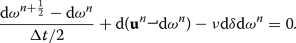 (153)
(153) -
Next, \(\omega ^{{n}+1}\) is computed with a semi-implicit scheme:
 (154)
(154) -
Equation (152c) is solved with an implicit scheme
$$\begin{aligned} \frac{{\theta }^{n+1}-{\theta }^n}{{\Delta }t}-{\delta } (\omega ^{n+\frac{1}{2}}\wedge {\theta }^{n+1})+{\kappa }{\delta }{\text {d}}{\theta }^{n+1} = 0. \end{aligned}$$(155)


Equations (153) and (154) are not solved directy for \(\omega ^{n+\frac{1}{2}}\) and \(\omega ^{n+1}\) but for the stream function \({\psi }^{n+\frac{1}{2}}\) and \({\psi }^{n+1}\). Indeed, since \({\delta }\omega =0\), the form \(\star \omega \) is exact. By Poincaré’s lemma, there is a 0-form \({\psi }\), the usual stream function, such that
Boundary conditions have to be provided for \({\psi }\).
Whenever needed, the dynamic pressure \(\overline{p}=p+\tfrac{1}{2}{\rho }||{\mathbf u}||^2\) can be computed by applying the operator \({\delta }\) on Eq. (152a):

Note that applying \({\delta }\) on (152a) is the counterpart, in tensor calculus, of the application of the divergence operator to the momentum equation in (151). So, if \({{\mathrm{div}}}\,{{\mathrm{curl}}}\) were not exactly zero, then the resolution of (157) would introduce an additional spurious pressure. In DEC, since \({\text {d}}^2\) is exactly zero, there is no such spurious pressure.
In space, a discretization with DEC is used. \({\psi }\) and \({\theta }\) are placed on primal vertices (the velocity form \(\omega \) is then on dual edges). The pressure is placed on the dual vertices.
Numerical tests
The first numerical example is a 2D channel flow. The length of the channel is \(L=2{\pi }\) and its height is \(H=1\). The viscosity is set to \({\nu }=1\) and the diffusivity to \({\kappa }=1\).
A zero flow is given as initial condition. The value of \({\theta }\) at the top wall is set to 20 and at the bottom wall and the inlet to 0. The grid is composed of 2744 triangles. The mean length of the edges is \(\Delta x_{mean}=2.989{\cdot }10^{-2}\). The time step is \({\Delta }t=10^{-2}\).
The computed velocity at \(t=5s\) is presented in Fig. 30, left. As can be observed, the computed profile is matches the exact one. The average absolute error is about \(2.4{\cdot }10^{-4}\).

Velocity (left) and \({\theta }\) (right) profile at \(x=3L/4\)
Figure 31 presents the magnitude of \({\theta }\) and some iso-contours. It shows the evolution of \({\theta }\) along the flow. In particular, it can be observed that \({\theta }\) has a linear profile, like the exact solution, in the fully developped region downstream the flow. It is confirmed by Fig. 30, right.

Repartition of the passive scalar
For the numerical analysis of convergence, Couette and Poiseuille flows were simulated, with \({\Delta }x_{mean}{\cdot }10^2=8.408\), 4.917, 2.091, 1.393, 1.044, 0.8354 and 0.6961, in a square domain. For primal 0-cochain \(\omega \) (stream function and temperature), the discrete norm is defined as
It corresponds to the usual \(L^2\) norm for a 0-form which is constant inside each dual cell. This definition is used instead of the usual \(L^2\) norm of the reconstructed form \(\hat{\omega }\) because it is easier to compute.
For dual 0-forms (such as the pressure), the following norm is used for the error analysis:
For dual 1-forms (like the flux v), we use the edge-based norm:
Figure 32 shows the evolution of the error with the grid size. As can be observed, the rate of convergence of the stream function \({\psi }\) is about 1.84. The temperature converges with a second order rate. The flux and the velocity are first order while the pressure convergence rate is 1.65.
For the Poiseuille flow, the convergence rate of the stream function is 1.37, as shown on Fig. 33. For the temperature, it is about 1.95. The flux and the velocity are first order as in [112]. Figure 34 shows the evolution of the discrete norm of \({\delta }v\) with time. As can be seen, \({\delta }v\) remains below the machine precision (about \(2{\cdot }10^{-16}\)), as well for the Couette flow as for the Poiseuille flow. This is due to the fact that, with DEC, \({\text {d}}^2=0\) at machine precision. As a consequence, the incompressibility condition (152b) is verified exactly, as well localy as globally.

Couette flow: Relative error on vorticity \({\psi }\), temperature \({\theta }\), flux v and velocity u, and absolute error \(E_d\) on dynamic pressure \(\overline{p}\)

Poiseuille flow: Relative error on vorticity \({\psi }\), temperature \({\theta }\), flux v, dynamical pressure and velocity u

Evolution of \({\delta }v\) with time. Top: Couette flow. Bottom: Poiseuille flow
To show the potential of DEC in predicting more realistic problems, we deal, in what follows, with the convection of a polluant in a ventilated room. The room geometry is presented in Fig. 35. The aspect ratio is set to \(L/H=1\). The height of the inlet and outlet is \(h=H/5\).
A polluted air flow, with a parabolic profile, is injected at the inlet. The Reynolds number based on centerline velocity and h is 100. The polluant is carbon dioxyde, with \({\theta }=1000\) at the inlet. At walls, \({\theta }=0\) (polluant particles which stick to the wall are extracted).

Ventilated-room geometry
The grid, composed of 3436 vertices and 6670 acute triangles, is presented in Fig. 36. The return period \({\tau }\), that is the time needed to cross a distance equal to the perimeter of the room with the inlet centerline velocity, is taken as time unit. The time step is set to \(2.10^{-3}{\tau }\). Some velocity streamlines and the repartition of the passive scalar are plotted in Fig. 37. This figure shows the evolution of the velocity and \({\theta }\) at \(t=0.5\), 1 and \(2{\tau }\).

Room grid

Velocity streamlines (left) and repartition of polluant (right), at, from top to bottom, \(t=0.5{\tau }\), \(t={\tau }\) and \(t=2{\tau }\)
DEC, as presented here, is used only as a spatial discretization method. The canonical metric of the space is used to define the discrete Hodge operator. This can easily be extended to a discretization on a Riemanian surface [213]. Extension to space-time is possible. For example, for the exterior calculus discretization of problems in gauge theory, the Hodge operator has been defined in [244] relatively to the Minkowski metric. An application to general relativity is presented in [245].
Conclusion
With this article, we aimed at raising the awarness among the readers, and particularly among high-performance computing specialists, about the importance of the geometric structure of their equations. This structure traduces fundamental physical properties and its preservation at the discrete level leads to robust numerical schemes.
Without being exhaustive, we tried to give an overview of the most popular geometric structures met in mechanics. For each of them, we presented a way to build a corresponding structure-preserving integrator.
Firstly, for Hamiltonian problems, we showed that symplectic integrators are particularly robust for long-time evolution problems. Their error on the energy of the system is bounded over an exponentially large time interval. More generally, symplectic integrators present generally good properties towards the preservation of conservation laws.
In the case of Hamiltonian PDEs, we presented a way of constructing multisymplectic integrators. It was shown that these multisymplectic schemes are more robust regarding the grid, in the sense that they allow more freedom in the choice of time and space steps, compared to classical schemes.
When the equations derive from a variational principle, we showed in section that with total variation approach, discrete energy and momentum evolution equations are obtained naturally, along with the Euler–Lagrange equation. We then presented a way to build variational integrators for ODEs and PDEs. We observed that, when the Lagrangian is time independent, these schemes preserve exactly the energy.
For more general equations, with or without symplectic or variational structure, we presented invariant schemes which preserve the Lie symmetry group of the equation. We saw that, contrarily to classical schemes, they do not introduce unphysical oscillations in presence of a pseudo-shock solution. They also do not give rise to spurious solution when the grid undergoes a Galilean transformation.
At last, we presented DEC which is a space integrator based on exterior calculus and which reproduces exactly Stokes theorem and the relation \({\text {d}}^2=0\) at the discrete scale. The second property enables, for example, to verify exactly the incompressibility condition. This also ensures the exact preservation of circulation in an ideal incompressible fluid flow. The use of DEC in mechanics being very recent, we presented some applications in fluid mechanics with passive scalar convection.
Other geometry-based integrators exist. We can cite, for instance, algorithms built to preserve a Lie–Poisson structure on a discrete manifold [246, 247]. Other examples are schemes based on a port-Hamiltonian, or more generally, on a Dirac structure, which aim at correctly handling the interconnection between subsystems [248]. Note that a combination of port Hamiltonian structure and DEC has been considered in [249]. Lie-group integrators can also be cited [250].
Notes
The interior product or contraction of a vector field \({\mathbf {X}}\) and a differential form \({\mu }\) is often noted \(i_{{\mathbf {X}}}\omega \) instead of
 . It is defined as
 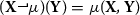 if \(\mu \) is a 2-form and \({\mathbf {Y}}\) any vector field.
The pull-back of \(\omega \) is defined as \(({\Phi }_t^*\omega )_{|\mathbf {s}}({\mathbf {X}}^1,{\mathbf {X}}^2)=\omega _{|{\Phi }_t(\mathbf {s})}\left( {{\text {d}}{\Phi }_{t}}_{|\mathbf {s}}({\mathbf {X}}^1),{{\text {d}}{\Phi }_t}_{|\mathbf {s}}({\mathbf {X}}^2)\right) \) for any pair of vector fields \({\mathbf {X}}^1\) and \({\mathbf {X}}^2\), \({\text {d}}{\Phi }_t\) being the differential of \({\Phi }_t\).
The exterior product of two differential 1-forms \(\omega ^1\) and \(\omega ^2\) is defined as the two form \((\omega ^1\wedge \omega ^2)({\mathbf {X}}^1,{\mathbf {X}}^2)=\omega ^1({\mathbf {X}}^1)\omega ^2({\mathbf {X}}^2)-\omega ^1({\mathbf {X}}^2)\omega ^2({\mathbf {X}}^1)\) for any pair of vector fields \({\mathbf {X}}^1\) and \({\mathbf {X}}^2\). More generally, the exterior product of a k-form \({\alpha }\) and a l-form \({\beta }\) is defined as the \((k+l)\)-form [147]:
\({\alpha }\wedge {\beta }({\mathbf {X}}^1,\ldots ,{\mathbf {X}}^{k+l})=\frac{1}{k!l!}\sum _{{\tau }\in S_{k+l}}{\text {sign}}({\tau })\ {\alpha }({\mathbf {X}}^{{\tau }(1)},\ldots ,{\mathbf {X}}^{{\tau }(k)})\ {\beta }({\mathbf {X}}^{{\tau }(k+1)},\ldots ,{\mathbf {X}}^{{\tau }(k+l)})\) for any vector fields \({\mathbf {X}}^1,\ldots ,{\mathbf {X}}^{k+l}\), \(S_{k+l}\) being the permutation group of \(\{1,\ldots ,k+l\}\).
More precisely,
$$\begin{aligned} \omega =\frac{1}{2}\sum _{i=1}^{n_{\mathbf {s}}}{\text {d}}s_i\wedge \bigg ( \sum _{j=1}^{n_{\mathbf {s}}} W_{ij}{\text {d}}s_j\bigg ) \end{aligned}$$if the \(W_{ij}\) are the components of \(\mathbb W\). Moreover, \(\displaystyle \omega ({\mathbf {X}}^1,{\mathbf {X}}^2)=(\mathbb W{\mathbf {X}}^1){\cdot }{\mathbf {X}}^2\) for two arbitrary vectors \({\mathbf {X}}^1\) and \({\mathbf {X}}^2\) of \( \mathbb {R}^{n_{\mathbf {s}}}\), the dot symbol \({\cdot }\) being the Euclidean inner product of \({\mathbb {R}}^{n_{\mathbf {s}}}\). Similar remarks apply to \({\kappa }\).
More rigorously, \(\mathcal M\) should be a fibre bundle with base \(\mathcal Z\) and a typical fiber \(\mathcal U\). The Lagrangian function is then defined in the jet bundle.
More precisely, \({\Omega }_k(K)\) is a \(\mathbb Z\)-module.
 . It is defined as
  if
if References
Marsden J, Ratiu T. Introduction to mechanics and symmetry. A basic exposition of classical mechanical systems. 2nd ed., Texts in applied mathematicsNew York: Springer; 1999.
Puta M. Hamiltonian mechanical systems and geometric quantization., Mathematics and its applicationsDordrecht: Springer Science and Business Media; 1993.
Deriglazov A. Classical mechanics: Hamiltonian and Lagrangian formalism. Berlin: Springer; 2017.
Hairer W, Wanner G, Lubich C. Geometric numerical integration. Structure-preserving algorithms for ordinary differential equations. 2nd ed., Springer series in computational mathematicsNew York: Springer; 2006.
Ruth RD. A canonical integration technique. IEEE Trans Nucl Sci. 1983;30(4):2669–71.
Channell PJ. Symplectic integration of Hamiltonian systems. Nonlinearity. 1990;3:231–59.
Kang F. Difference schemes for Hamiltonian formalism and symplectic geometry. J Comput Math. 1986;4(3):279–89.
Menyuk C. Some properties of the discrete Hamiltonian method. Physica D Nonlin Phenomena. 1984;11(1):109–29.
Hairer W, Norsett SP, Wanner G. Solving ordinary differential equations I: nonstiff problems. Berlin: Springer; 1987.
Lasagni FM. Canonical Runge–Kutta methods. Zeitschrift für angewandte Mathematik und Physik. 1988;39(6):952–3.
Sanz-Serna JM. Runge–Kutta schemes for Hamiltonian systems. BIT Numer Math. 1988;28(4):877–83.
Suris Y. Hamiltonian methods of Runge–Kutta type and their variational interpretation. Matem Mod. 1990;2(4):78–87.
Marsden J, West M. Discrete mechanics and variational integrators. Acta Numerica. 2001;10:57–514.
West M. Variational integrators, Ph.D. Thesis. California Institute of Technology; 2004.
Mata P, Lew AJ. Variational integrators for the dynamics of thermo-elastic solids with finite speed thermal waves. J Comput Phys. 2014;257(Part B):1423–43.
Ma Y, Kong L, Hong J, Cao Y. High-order compact splitting multisymplectic method for the coupled nonlinear Schrödinger equations. Comput Math Appl. 2011;61(2):319–33.
Wang D, Xiao A. Fractional variational integrators for fractional variational problems. Commun Nonlin Sci Numer Simul. 2012;17(2):602–10.
Ober-Blöbaum S, Tao M, Cheng M, Owhadi H, Marsden JE. Variational integrators for electric circuits. J Comput Phys. 2013;242(Supplement C):498–530.
Liao C, Shen W, Ding X. Multi-symplectic variational integrators for the Gross–Pitaevskii equations in BEC. Appl Math Lett. 2016;60(Supplement C):120–5.
Kraus M, Tassi E, Grasso D. Variational integrators for reduced magnetohydrodynamics. J Comput Phys. 2016;321(Supplement C):435–58.
Li Y, Wu B, Leok M. Spectral variational integrators for semi-discrete Hamiltonian wave equations. J Comput Appl Math. 2017;325(Supplement C):56–73.
Li Y, Wu B, Leok M. Spectral-collocation variational integrators. J Comput Phys. 2017;332(Supplement C):83–98.
Kraus M. Variational integrators in plasma physics, Ph.D. thesis. Technische Universität Mu\(\ddot{{\rm n}}\)chen; 2013.
Kraus M, Maj O. Variational integrators for nonvariational partial differential equations. Physica D Nonlin Phenomena. 2015;310(Supplement C):37–71.
Gallissot F. Les formes extérieures et la mécanique des milieux continus. Annales de l’Institut Fourier. 1958;8:291–335.
Gotay MJ. A multisymplectic framework for classical field theory and the calculus of variations: I. Covariant Hamiltonian formalism. In: Francaviglia M, editor. Mechanics, analysis and geometry: 200 years after lagrange., North-Holland delta seriesAmsterdam: Elsevier; 1991. p. 203–35.
Gotay MJ. A multisymplectic framework for classical field theory and the calculus of variations II: space + time decomposition. Differ Geom Appl. 1991;1(4):375–90.
Dedecker P. On the generalization of symplectic geometry to multiple integrals in the calculus of variations. In: Bleuler K, Reetz A, editors. Differential geometrical methods in mathematical physics: proceedings of the symposium held at the university of Bonn, July 1–4, 1975. Lecture notes in mathematics. Berlin: Springer; 1977. p. 395–456.
Gawdzki K. On the geometrization of the canonical formalism in the classical field theory. Rep Math Phy. 1972;3(4):307–26.
Goldschmidt H, Sternberg S. The Hamilton–Cartan formalism in the calculus of variations. Annales de l’Institut Fourier. 1973;23(1):203–67.
Kijowski J. A finite-dimensional canonical formalism in the classical field theory. Commun Math Phys. 1973;30(2):99–128.
Günther C. The polysymplectic Hamiltonian formalism in field theory and calculus of variations. I. The local case. J Differ Geom. 1987;25(1):23–53.
Cariñena JF, Crampin M, Ibort LA. On the multisymplectic formalism for first order field theories. Differ Geom Appl. 1991;1(4):345–74.
Awane A. K-symplectic structures. J Math Phys. 1992;12:33.
Giachetta G, Mangiarotti L, Sardanashvily G. New Lagrangian and Hamiltonian methods in field theory. Singapore: World Scientific; 1997.
McLean M, Norris LK. Covariant field theory on frame bundles of fibered manifolds. AIP J Math Phys. 2000;41:6808–23.
León M, Salgado M, Vilarino S. Methods of differential geometry in classical field theories: \(k\)-symplectic and \(k\)-cosymplectic approaches. Singapore: World Scientific Publishing; 2015.
García PL, Pérez-Rendón A. Symplectic approach to the theory of quantized fields. I. Commun Math Phys. 1969;13(1):24–44.
Cantrijn F, Ibort A, De León M. On the geometry of multisymplectic manifolds. J Aust Math Soc Ser A Pure Math Stat. 1999;66(3):303–30.
Román-Roy N, Salgado M, Vilariño S. Symmetries and conservation laws in the Günther \(k\)-symplectic formalism of field theory. Rev Math Phys. 2007;19(10):1117–47.
Bua L, Bucataru I, Salgado M. Symmetries, Newtonoids vector fields and conservation laws in the Lagrangian \(k\)-symplectic formalism. Rev Math Phys. 2012;24(10):1250030.
Marrero JC, Román-Roy N, Salgado M, Vilariño S. On a kind of Nœther symmetries and conservation laws in \(k\)-cosymplectic field theory. J Math Phys. 2011;52(2):022901.
Herman J. Noether’s theorem in multisymplectic geometry. Differ Geom Appl. 2018;56:260–94.
Bridges T, Derks G. Unstable eigenvalues and the linearization about solitary waves and fronts with symmetry. Proc Math Phys Eng Sci. 1999;455(1987):2427–69.
Frank J. Geometric space-time integration of ferromagnetic materials. Appl Numer Math. 2004;48(3):307–22.
Chen JB. Multisymplectic geometry, local conservation laws and a multisymplectic integrator for the Zakharov–Kuznetsov equation. Lett Math Phys. 2003;63(2):115–24.
Bridges T, Reich S. Multi-symplectic spectral discretizations for the Zakharov–Kuznetsov and shallow water equations. Physica D Nonlin Phenomena. 2001;152–153:491–504.
Cotter C, Holm D, Hydon P. Multisymplectic formulation ef fluid dynamics using the inverse map. Proc R Soc A. 2007;463:2671–87.
Li H, Sun J. A new multi-symplectic Euler box scheme for the “BBM” equation. Math Comput Model. 2013;58(7–8):1489–501.
Cai W, Wang Y, Song Y. Derivation of the multisymplectic Crank–Nicolson scheme for the nonlinear Schrödinger equation. Comput Phys Commun. 2014;185(10):2403–11.
Kong L, Hong J, Zhang J. Splitting multisymplectic integrators for Maxwell’s equations. J Comput Phys. 2010;229(11):4259–78.
Chen JB. A multisymplectic pseudospectral method for seismic modeling. Appl Math Comput. 2007;186(2):1612–6.
Ascher UM, McLachlan RI. Multisymplectic box schemes and the Korteweg–de Vries equation. Appl Numer Math. 2004;48(3):255–69.
Olver P. Applications of Lie groups to differential equations., Graduate texts in mathematicsNew York: Springer; 1986.
Ibragimov NH. CRC handbook of Lie group analysis of differential equations., Symmetries, exact solutions and conservation lawsBoca Raton: CRC Press; 1994.
Ibragimov NH. CRC handbook of Lie group analysis of differential equations., Applications in engineering and physical sciencesBoca Raton: CRC Press; 1995.
Ibragimov NH. CRC handbook of Lie group analysis of differential equations., New trends in theoretical developments and computational methodsBoca Raton: CRC Press; 1996.
Grassi V, Leo RA, Soliani G, Tempesta P. Vorticies and invariant surfaces generated by symmetries for the 3D Navier–Stokes equation. Physica A. 2000;286:79–108.
Zhao Z, Han B. Lie symmetry analysis of the Heisenberg equation. Commun Nonlin Sci Numer Simul. 2017;45(Supplement C):220–34.
Bozhkov Y, Dimas S, Ibragimov NH. Conservation laws for a coupled variable-coefficient modified Korteweg–de Vries system in a two-layer fluid model. Commun Nonlin Sci Numer Simul. 2013;18(5):1127–35.
Yaşar E, Özer T. On symmetries, conservation laws and invariant solutions of the foam-drainage equation. Int J Nonlin Mech. 2011;46(2):357–62.
Wang G, Kara AH. Nonlocal symmetry analysis, explicit solutions and conservation laws for the fourth-order Burgers’ equation. Chaos Solitons Fractals. 2015;81(Part A):290–8.
Wang JY, Tang XY, Liang ZF, Lou SY. Infinitely many nonlocal symmetries and conservation laws for the (1+1)-dimensional Sine–Gordon equation. J Math Anal Appl. 2015;421(1):685–96.
Inc M, Aliyu AI, Yusuf A. Solitons and conservation laws to the resonance nonlinear Shrödinger’s equation with both spatio-temporal and inter-modal dispersions. Optik Int J Light Etectron Opt. 2017;142(Supplement C):509–22.
Cao Z, Lin Y, Shen J. Conservation laws for a variable coefficient nonlinear diffusion-convection-reaction equation. J Math Anal Appl. 2014;420(1):77–93.
Gandarias ML, Bruzón MS, Rosa M. Nonlinear self-adjointness and conservation laws for a generalized Fisher equation. Commun Nonlin Sci Numer Simul. 2013;18(7):1600–6.
Ibragimov NH. Conservation laws and non-invariant solutions of anisotropic wave equations with a source. Nonlin Anal Real World Appl. 2018;40(Supplement C):82–94.
Jhangeer A. Conservation laws for the (1+2)-dimensional wave equation in biological environment. Acta Mathematica Scientia. 2013;33(5):1255–68.
Oberlack M. A unified approach for symmetries in plane parallel turbulent shear flows. J Fluid Mech. 2001;427:299–328.
Oberlack M. On the decay exponent of isotropic turbulence. PAMM. 2002;1:294–7.
Lindgren B, Österlund J, Johansson A. Evaluation of scaling laws derived from Lie group symmetry methods in zero-pressure-gradient turbulent boundary layers. J Fluid Mech. 2004;502:127–52.
Oberlack M, Cabot W, Pettersson Reif B, Weller T. Group analysis, direct numerical simulation and modelling of a turbulent channel flow with streamwise rotation. J Fluid Mech. 2006;562:355–81.
Razafindralandy D, Hamdouni A, Oberlack M. Analysis and development of subgrid turbulence models preserving the symmetry properties of the Navier–Stokes equations. Eur J Mech B. 2007;26:531–50.
Razafindralandy D, Hamdouni A, Chhay M, Razafindralandy D, Hamdouni A, Chhay M. Symmetry in turbulence simulation. In: Colombo S, Rizzo C, editors. Numerical simulation research progress. New York: Nova Publishers; 2009. p. 161–207.
Sayed NA, Hamdouni A, Liberge E, Razafindralandy D. The symmetry group of the non-isothermal Navier–Stokes equations and turbulence modelling. Symmetry. 2010;2:848–67.
Razafindralandy D, Hamdouni A, Sayed NA. Lie-symmetry group and modeling in non-isothermal fluid mechanics. Physica A Stat Mech Appl. 2012;391(20):4624–36.
Dorodnitsyn VA. Finite difference models entirely inheriting continuous symmetry of original differential equations. Int J Mod Phys C. 1994;05(04):723–34.
Welk M, Kim P, Olver PJ. Numerical invariantization for morphological PDE schemes. In: Sgallari F, Murli A, Paragios N, editors. Scale space and variational methods in computer vision: first international conference, SSVM 2007, Ischia, Italy, May 30–June 2, 2007. Proceedings. Berlin: Springer; 2007. p. 508–19.
Kim P. Invariantization of numerical schemes using moving frames. BIT Numer Math. 2007;47(3):525–46.
Chhay M, Hamdouni A. A new construction for invariant numerical schemes using moving frames. Comptes Rendus Mécanique. 2010;338(2):97–101.
Chhay M, Hoarau E, Hamdouni A, Sagaut P. Comparison of some Lie-symmetry-based integrators. J Comput Phys. 2011;230(5):2174–88.
Rebelo R, Valiquette F. Symmetry preserving numerical schemes for partial differential equations and their numerical tests. J Differ Equ Appl. 2013;19(5):738–57.
Budd C, Dorodnitsyn V. Symmetry-adapted moving mesh schemes for the nonlinear Schrödinger equation. J Phys A Math Gen. 2001;34(48):10387.
Electromagnetics Deschamps G, Forms Differential. Electromagnetics and differential forms. Proc IEEE. 1981;69(6):676–96.
Griffiths P, Bryant R, Hsu L. Hyperbolic exterior differential systems and their conservation laws. I. Selecta Mathematica New Ser. 1995;1(1):21–112.
Griffiths P, Bryant R, Hsu L. Hyperbolic exterior differential systems and their conservation laws. II. Selecta Mathematica New Ser. 1995;1(2):265–323.
Tonti E. Why starting from differential equations for computational physics? J Comput Phys. 2014;257(Part B):1260–90.
Bossavit A. Computational electromagnetism. Variationl formulations, complementarity, edge elements. In: Mayergoyz I, editor. Electromagnetism. New York: Academic Press; 1998.
Bossavit A. On the geometry of electromagnetism: (1) Affine space. J Jpn Soc Appl Electromagn Mech. 1998;6:17–28.
Bossavit A. On the geometry of electromagnetism: (2) geometrical objects. J Jpn Soc Appl Electromagn Mech. 1998;6:114–23.
Bossavit A. On the geometry of electromagnetism: (3) integration, Stokes, Faraday’s law. J Japn Soc Appl Electromagn Mech. 1998;6:233–40.
Bossavit A. On the geometry of electromagnetism: (4) Maxwell’s house. J Jpn Soc Appl Electromagn Mech. 1998;6:318–26.
Tonti E. The reason for analogies between physical theories. Appl Math Model. 1976;1(1):37–50.
Tonti E. The mathematical structure of classical and relativistic physics: a general classification diagram. Basel: Birkhäuser; 2013.
Hymann J, Scovel J. Deriving mimetic difference approximations to differential operators using algebraic topology, technical report. Los Alamos National Laboratory; 1990.
Mattiussi C. An analysis of finite volume, finite element, and finite difference methods using some concepts from algebraic topology. J Comput Phys. 1997;133(2):289–309.
Adams D. R-torsion and linking numbers from simplicial Abelian gauge theories. arXiv:hep-th/9612009. 1996.
Sen S, Sen S, Sexton J, Adams D. Geometric discretization scheme applied to the Abelian Chern–Simons theory. Phys Rev E. 2000;61(3):3174–85.
Bossavit A. Computational electromagnetism and geometry: (1) network equations. J Jpn Soc Appl Electromagn Mech. 1999;7(2):150–9.
Bossavit A. Computational electromagnetism and geometry: (2) network constitutive laws. J Jpn Soc Appl Electromagn Mech. 1999;7(3):204–301.
Bossavit A. Computational electromagnetism and geometry : (3): convergence. J Jpn Soc ApplElectromagn Mech. 1999;7(4):401–8.
Bossavit A. Computational electromagnetism and geometry : (4): from degrees of freedom to fields. J Jpn Soc Appl Electromagn Mech. 2000;8(1):102–9.
Bossavit A. Computational electromagnetism and geometry : (5): the Galerkin Hodge. J Jpn Soc Appl Electromagn Mech. 2000;8(2):203–9.
Bossavit A. Generalized finite differences in computational electromagnetics. Progr Electromagn Res. 2001;32:45–64.
Bossavit A. Discretization of electromagnetic problems: the “generalized finite differences” approach. In: Schilders WHA, editor. Numerical methods in electromagnetics. Handbook of numerical analysis. Amsterdam: Elsevier; 2005. p. 105–97.
Chen SC, Chew WC. Numerical electromagnetic frequency domain analysis with discrete exterior calculus. J Comput Phys. 2017;350(Supplement C):668–89.
Räbinä J, Mönkölä S, Rossi T, Penttilä A, Muinonen A. Comparison of discrete exterior calculus and discrete-dipole approximation for electromagnetic scattering. J Quant Spectrosc Radiat Transf. 2014;146(Supplement C):417–23.
Xie Z, Ye Z, Ma YJ. Numerical simulation of antennae by discrete exterior calculus. Commun Theor Phys. 2009;52(6):1067.
Ye Z, Xie Z, Ma YJ. Numerical simulation of electromagnetic waves scattering by discrete exterior calculus. Chin Phys Lett. 2009;26(8):084102.
Elcott S, Tong Y, Kanso E, Schröder P, Desbrun M. Stable, circulation-preserving, simplicial fluids. ACM Trans Graph. 2007;26(1):4.
Hirani A, Nakshatrala K, Chaudhry J. Numerical method for Darcy flow derived using discrete exterior calculus. Int J Comput Methods Eng Sci Mech. 2015;16:151–69.
Mohamed M, Hirani A, Samtaney R. Discrete exterior calculus discretization of incompressible Navier–Stokes equations over surface simplicial meshes. J Comput Phys. 2016;312:175–91.
Yavari A. On geometric discretization of elasticity. J Math Phys. 2008;49(2):022901.
Angoshtari A, Yavari A. A geometric structure-preserving discretization scheme for incompressible linearized elasticity. Comput Methods Appl Mech Eng. 2013;259(Supplement C):130–53.
Seslija M, van der Schaft A, Scherpen J. Discrete exterior geometry approach to structure-preserving discretization of distributed-parameter port-Hamiltonian systems. J Geom Phys. 2012;62(6):1509–31.
Bochev P, Hyman J. Principles of mimetic discretizations of differential operators. In: Arnold D, Bochev P, Lehoucq R, Nicolaides R, Shashkov M, editors. Compatible spatial discretizations., The IMA volumes in mathematics and its applicationsNew York: Springer; 2006. p. 89–119.
Nicolaides A, Trapp K. Covolume discretization of differential forms. In: Arnold D, Bochev P, Lehoucq R, Nicolaides R, Shashkov M, editors. Compatible spatial discretizations., The IMA volumes in mathematics and its applicationsNew York: Springer; 2006. p. 161–71.
Hiemstra RR, Toshniwal D, Huijsmans RHM, Gerritsma MI. High order geometric methods with exact conservation properties. J Comput Phys. 2014;257(Part B):1444–71.
Kreeft J, Gerritsma M. Mixed mimetic spectral element method for Stokes flow: a pointwise divergence-free solution. J Comput Phys. 2013;240(Supplement C):284–309.
Kreeft J, Palha A, Gerritsma M. Mimetic framework on curvilinear quadrilaterals of arbitrary order. arXiv:1111.4304; 2011.
Palha A, Gerritsma M. A mass, energy, enstrophy and vorticity conserving (MEEVC) mimetic spectral element discretization for the 2D incompressible Navier–Stokes equations. J Comput Phys. 2017;328(Supplement C):200–20.
Rufat D, Mason G, Mullen P, Desbrun M. The chain collocation method: a spectrally accurate calculus of forms. J Comput Phys. 2014;257(Part B):1352–72.
Gross B, Atzberger P. Spectral numerical exterior calculus methods for radial manifolds. arXiv:1703.00996; 2017.
Arnold D, Falk R, Winther R. Finite element exterior calculus, homological techniques, and applications. Acta Numerica. 2006;15:1–155.
Arnold D, Falk R, Winther R. Finite element exterior calculus: from Hodge theory to numerical stability. Bull Am Math Soc. 2010;47:281–354.
Cotter CJ, Thuburn J. A finite element exterior calculus framework for the rotating shallow-water equations. J Comput Phys. 2014;257(Part B):1506–26.
Lipnikov K, Manzini G, Shashkov M. Mimetic finite difference method. J Comput Phys. 2014;257(Part B):1163–227.
Perot B. Conservation properties of unstructured staggered mesh schemes. J Comput Phy. 2000;159:58–89.
Castillo J, Miranda G. Mimetic discretization methods. Boca Raton: CRC Press; 2013.
Lipnikov K, Reynolds J, Nelson E. Mimetic discretization of two-dimensional magnetic diffusion equations. J Comput Phys. 2013;247(Supplement C):1–16.
Back A, Sonnendrücker E. Finite element Hodge for spline discrete differential forms. Application to the Vlasov–Poisson system. Appl Numer Math. 2014;79(Supplement C):124–36.
Back A, Sonnendrücker E. Spline discrete differential forms. Application to Maxwell’s equations; 2011. https://hal.archives-ouvertes.fr/hal-00568811.
Kim P. Invariantization of the Crank–Nicolson method for Burgers’ equation. Physica D Nonlin Phenomena. 2008;237(2):243–54.
Leon M, Rodrigues P. Methods of differential geometry in analytical mechanics. Amsterdam: Elsevier Science Publishers; 1989.
Olver P. Moving frames. J Symb Comput. 2003;36(3–4):501–12.
Epstein M. The geometrical language of continuum mechanics. Cambridge: Cambridge University Press; 2010.
Spivak M. A comprehensive introduction to differential geometry. 3rd ed. Houston: Publish or Perish; 1999.
Spivak M. A comprehensive introduction to differential geometry. 3rd ed. Houston: Publish or Perish; 1999.
Spivak M. A comprehensive introduction to differential geometry. 3rd ed. Houston: Publish or Perish; 1999.
Spivak M. A comprehensive introduction to differential geometry. 3rd ed. Houston: Publish or Perish; 1999.
Spivak M. A comprehensive introduction to differential geometry. 3rd ed. Houston: Publish or Perish; 1999.
Isham CJ. Modern differential geometry for physicists., World scientific lecture note in physicsSingapore: World Scientific; 1999.
Burke W. Applied differential geometry. Cambridge: Cambridge University Press; 1985.
McDuff D, Salamon D. Introduction to symplectic topology. 2nd ed., Oxford mathematical monographsOxford: Oxford University Press; 1998.
da Silva AC. Lectures on symplectic geometry., Lecture notes in mathematicsBerlin: Springer; 2008.
Arnold VI. Mathematical methods of classical mechanics. 2nd ed., Graduate texts in mathematicsNew York: Springer; 1989.
Abraham R, Marsden JE, Ratiu R. Manifolds, tensor analysis, and applications. New York: Springer; 1988.
Goldstein H. Classical mechanics. 2nd ed., Addison-Wesley series in physicsBoston: Addison-Wesley Publication; 1980.
Goldstein H, Poole C, Safko J. Classical mechanics. 3rd ed. Harlow: Pearson; 2001.
Haier E, Lubich C, Wanner G. Geometric Numerical integration: structure-preserving algorithms for ordinary differential equations. 2nd ed. New York: Springer; 2006.
Sanz-Serna JM. Symplectic integrators for Hamiltonian problems: an overview. Acta Numerica. 1992;1:243–86.
Feng K, Qin M. Symplectic geometric algorithms for Hamiltonian systems. Berlin: Springer; 2010.
Sun G. A simple way constructing symplectic Runge–Kutta methods. J Comput Math. 2000;18(1):61–8.
Kang F, Hua-mo W, Qin M, Wang D. Construction of canonical difference schemes for Hamiltonian formalism via generating functions. J Comput Math. 1989;7(1):71–96.
Leimkuhler B, Reich S. Simulating Hamiltonian dynamics., Cambridge monographs on applied and computational mathematicsCambridge: Cambridge University Press; 2004.
Ge Z, Marsden JE. Lie–Poisson Hamilton–Jacobi theory and Lie–Poisson integrators. Phys Lett A. 1988;133:134–9.
Benettin G, Giorgilli A. On the Hamiltonian interpolation of near-to-the identity symplectic mappings with application to symplectic integration algorithms. J Stat Phys. 1994;74(5):1117–43.
Hairer E, Lubich C. The life-span of backward error analysis for numerical integrators. Numerische Mathematik. 1997;76(4):441–62.
Cooper GJ. Stability of Runge–Kutta methods for trajectory problems. IMA J Numer Anal. 1987;7(1):1–13.
Chartier P, Hairer E, Vilmart G. Numerical integrators based on modified differential equations. Math Comput. 2007;76(260):1941–53.
Yoshida H. Non-existence of the modified first integral by symplectic integration methods II: Kepler problem. Celesti Mech Dyn Astronomy. 2002;83:355–64.
Minesaki Y, Nakamura Y. A new discretization of the Kepler motion which conserves the Runge–Lenz vector. Phys Lett A. 2002;306(2):127–33.
Waldvogel J. A new regularization of the planar problem of three bodies. J Celest Mech. 1972;6:221.
Aref H, Pomphrey N. Integrable and chaotic motions of four vortices. Phys Lett A. 1980;78(4):297–300.
Lamb H. Hydrodynamics. Cambridge: University Press; 1916.
Aref H. Point vortex dynamics: a classical mathematics playground. J Math phys. 2007;48:065401.
Newton PK. Point vortex dynamics in the post-Aref era. Fluid Dyn Res. 2014;46(3):031401.
Boatto G, Pierrehumbert R. Dynamics of a passive tracer in a velocity field of four identical point vortices. J Fluid Mech. 1999;394:137–74.
Bécu E, Pavlov V. Evolution of localized vortices in the presence of stochastic perturbations. Nonlin Process Geophys. 2006;13(1):41–51.
Chhay M. Intégrateurs géométriques: application à la mécanique des fluides, Ph.D. Thesis. Université de La Rochelle; 2008.
Bridges T. Multi-symplectic structures and wave propagation. Math Proc Camb Philos Soc. 1997;121:147.
Dutykh D, Clamond D, Chhay M. Serre-type equations in deep water. Math Model Nat Phenom. 2017;12(1):23–40.
Chhay M, Dutykh D, Clamond D. On the multi-symplectic structure of the Serre–Green–Naghdi equations. J Phys A Math Theor. 2016;49(3):03LT01.
Dutykh D, Chhay M, Fedele F. Geometric numerical schemes for the KdV equation. Comput Math Math Phys. 2013;53(2):221–36.
Hélein F. Multisymplectic formalism and the covariant phase. In: Bielawski R, Houston K, Speight M, editors. Variational problems in differential geometry., London mathematical society lecture note seriesCambridge: Cambridge University Press; 2011. p. 94–126.
Bridges T, Reich S. Multi-symplectic integrators: numerical schemes for Hamiltonian PDEs that conserve symplecticity. Phys Lett A. 2001;284(4–5):184–93.
Moore B, Reich S. Backward error analysis for multi-symplectic integration methods. Numerische Mathematik. 2003;95(4):625–52.
Hong J, Liu H, Sun G. The multi-symplecticity of partitioned Runge–Kutta methods for Hamiltonian PDEs. Math Comput. 2005;75(253):167–81.
Ryland B, McLachlan R. On multisymplecticity of partitioned Runge–Kutta methods. SIAM J Sci Comput. 2008;30(3):1318–40.
Hu WP, Deng ZC, Han SM, Fa W. Multi-symplectic Runge–Kutta methods for Landau–Ginzburg–Higgs equation. Appl Math Mech. 2009;30(8):1027–34.
Reich S. Multi-symplectic Runge–Kutta collocation methods for Hamiltonian waveequations. J Comput Phys. 1999;157:473–99.
Li Q, Sun Y, Wang Y. On multisymplectic integrators based on Runge–Kutta–Nyström methods for Hamiltonian wave equations. Appl Math Comput. 2006;182(2):1056–63.
Hong J, Liu XY, Li C. Multi-symplectic Runge–Kutta–Nyström methods for nonlinear Schrödinger equations with variable coefficients. J Comput Phys. 2007;226(2):1968–84.
Wu X, You X, Wang B. Structure-preserving algorithms for oscillatory differential equations. Beijing: Springer and Science Press; 2013.
Duncan DB. Symplectic finite difference approximations of the nonlinear Klein–Gordon equation. SIAM J Numer Anal. 1997;34(5):1742–60.
Wang YS, Qin MZ. Multisymplectic schemes for the nonlinear Klein–Gordon equation. Math Comput Model. 2002;36(9–10):963–77.
Brizard AJ. An introduction to Lagrangian mechanics. Singapore: World Scientific; 2008.
Calkin MG. Lagrangian and Hamiltonian mechanics. Singapore: World Scientific; 1996.
Kane C, Marsden J, Ortiz M. Symplectic-energy-momentum preserving variational integrators. J Math Phys. 1999;40(7):3353–71.
Chen JB, Guo HY, Wu K. Discrete total variation calculus and Lee’s discrete mechanics. Appl Math Comput. 2006;177(1):226–34.
Nœther E. Invariante Variationsprobleme. Nachrichten von der Gesellschaft der Wissenschaften zu Göttingen: Mathematisch-Physikalische Klasse; 1918. p. 235–57.
Nœther E, Tavel A. Invariant variation problems. Transp Theory Stat Phys. 1971;1(3):183–207 (English traduction of the Nœther’s original paper [191]).
Kosmann-Schwarzbach Y. Les théorèmes de Nœther. Éditions de l’École Polytechnique; 2004.
Kosmann-Schwarzbach Y. The Noether theorems:invariance and conservation laws in the twentieth century., Sources and studies in the history of mathematics and physical sciencesNew York: Springer; 2011.
Chen JB. Variational integrators and the finite element method. Appl Math Comput. 2008;196(2):941–58.
Mütze U. Predicting classical motion directly from the action principle (II). 1999. https://www.ma.utexas.edu/mp_arc/c/99/99-271.pdf. Accessed 30 May 2018.
Mütze U. Predicting classical motion directly from the action principle (III). 2000. http://www.ulrichmutze.de/articles/01-166.ps. Accessed 30 May 2018.
Cano B, Lewis HR. A comparison of symplectic and Hamilton’s principle algorithms for autonomous and non-autonomous systems of ordinary differential equations. Appl Numer Math. 2001;39(3–4):289–306.
Nair S. Time adaptive variational integrators: a space-time geodesic approach. Physica D Nonlin Phenomena. 2012;241(4):315–25.
Shibberu Y. Time-discretization of Hamiltonian dynamical systems. Comput Math Appl. 1994;28(10):123–45.
Lewis HR, Kostelec PJ. The use of Hamilton’s principle to derive time-advance algorithms for ordinary differential equations. Comput Phys Commun. 1996;96(2):129–51.
Chen JB. Total variation in discrete multisymplectic field theory and multisymplectic-energy-momentum integrators. Lett Math Phys. 2002;61(1):63–73.
Baker A. Matrix groups: an introduction to Lie group theory., Springer undergraduate mathematics seriesLondon: Springer; 2002.
Hereman W. Review of symbolic software for the computation of Lie symmetries of differential equations. Euromath Bull. 1994;1(2):45–79.
Vu K, Carminati J. Symbolic computation and differential equations: Lie symmetries. J Symb Comput. 2000;29(2):95–116.
Cheviakov F. GeM software package for computation of symmetries and conservation laws of differential equations. Comput Phys Commun. 2007;176(1):48–61.
Cheviakov A. Symbolic computation of nonlocal symmetries and nonlocal conservation laws of partial differential equations using the GeM package for Maple. In: Ganghoffer JF, Mladenov I, editors. Similarity and symmetry methods: applications in elasticity and mechanics of materials., Lecture notes in applied and computational mechanicsCham: Springer International Publishing; 2014. p. 165–84.
Olver P. Geometric foundations of numerical algorithms and symmetry. Appl Algebra Eng Commun Comput. 2001;11(5):417–36.
Cartan E. La méthode de repère mobile, la théorie des groupes continus et les espaces généralisés. Hermann: Actualités Scientifiques et Industrielles; 1935.
Edelen D. Applied exterior calculus., Doverbooks on mathematicsMineola: Dover Publications; 2005.
Flanders H. Differential forms with applications to the physical sciences., Dover books on mathematicsNew York: Dover Publications; 1989.
Frankel T. The geometry of physics: an introduction. 3rd ed. Cambridge: Cambridge University Press; 2011.
Nitschke I, Reuther S, Voigt A. Discrete exterior calculus (DEC) for the surface Navier–Stokes equation. In: Bothe D, Reusken A, editors. Transport processes at fluidic interfaces. Advances in mathematical fluid. Cham: Birkhäuser; 2017. p. 177–97.
Hirani A. Discrete exterior calculus, Ph.D. Thesis. California Institute of Technology. Pasadena, CA, USA; 2003.
Pontryagin LS. Foundations of combinatorial topology. Rochester: Graylock Press; 1952 (Translated from the first (1947) Russian edition by Bagemihl. Seidel: Komm).
Wallace A. An introduction to algebraic topology. Dover Books on Mathematics. Mineola: Dover Publications; 2007.
Wallace A. Algebraic topology: homology and cohomology. Dover books on mathematics. Mineola: Dover Publications; 2007.
tom Dieck T. Algebraic topology., EMS textbooks in mathematicsZürich: European Methematical Society; 2008.
Shastri A. Basic algebraic topology. Hoboken: CRC Press; 2013.
Desbrun M, Hirani A, Leok M, Marsden J. Discrete exterior calculus. arXiv:math/0508341; 2005.
Gillette A. Notes on discrete exterior calculus. University of Texas at Austin; 2009.
Crane K, de Goes F, Desbrun M, Schröder P. Digital Geometry Processing with Discrete Exterior Calculus. In: ACM SIGGRAPH 2013 courses. SIGGRAPH ’13. ACM; 2013.
Arnold D, Bochev P, Lehoucq R, Nicolaides R, Shashkov M, editors. Compatible spatial discretizations., The IMA volumes in mathematics and its applicationsNew York: Springer; 2006.
Bonelle J. Compatible discrete operator schemes on polyhedral meshes for elliptic and Stokes equations, Ph.D. Thesis. Université Paris-Est; 2014.
Christiansen S, Munthe-Kaas H, Owren B. Topics in structure-preserving discretization. Acta Numerica. 2011;20:1–119.
Whitney H. Geometric integration theory. Princeton: Princeton University Press; 1957.
Bossavit A. Whitney forms: a class of finite elements for three-dimensional computations in electromagnetism. IEE Proc A Sci Meas Technol. 1988;135(8):493–500.
Bossavit A. A uniform rationale for Whitney forms on various supporting shapes. Math Comput Simul. 2010;80(8):1567–77.
Schulz E, Tsogtgerel G. Convergence of discrete exterior calculus approximations for Poisson problems. arXiv:1611.03955 [mathNA]; 2016.
Hiptmair R. Higher order Whitney forms. Progr Electromagn Res. 2001;32:271–99.
Rapetti F, Bossavit A. Whitney forms of higher degree. SIAM J Numer Anal. 2009;47(3):2369–86.
Yee K. Numerical solution of initial boundary value problems involving Maxwell’s equations in isotropic media. IEEE Trans Antennas Propag. 1966;14(3):302–7.
Hiptmair R. Discrete Hodge operators. Numerische Mathematik. 2001;90(2):265–89.
Hirani A, Kalyanaraman K, VanderZee E. Technical note: Delaunay Hodge star. ComputerAided Des. 2013;45(2):540–4.
Mullen P, Memari P, de Goes F, Desbrun M. HOT: Hodge-optimized triangulations. ACM Trans Graph. 2011;30(4):103:1–12.
Mohamed M, Hirani A, Samtaney R. Comparison of discrete Hodge star operators for surfaces. ComputerAided Des. 2016;78:118–25.
Tarhasaari T, Kettunen L, Bossavit A. Some realizations of a discrete Hodge operator: a reinterpretation of finite element techniques. IEEE Trans Magn. 1999;35(3):1494–7.
Bossavit A. Extrusion, contraction: their discretization via Whitney forms. Int J Comput Math Electr. 2003;22(3):470–80.
Mullen P, McKenzie A, Pavlov D, Durant L, Tong Y, Kanso E, et al. Discrete Lie advection of differential forms. Found Comput Math. 2011;11(2):131–49.
Demkowicz L, Monk P, Vardapetyan L, Rachowicz W. De Rham diagram for hp finite element spaces. Comput Math Appl. 2000;39(7):29–38.
Hiptmair R. Finite elements in computational electromagnetism. Acta Numerica. 2002;11:237–339.
Monk P. Finite element methods for Maxwell’s equations., Numerical mathematics and scientific computationOxford: Oxford University Press; 2003.
Story TL. Introduction to differential geometry with applications to Navier–Stokes dynamics. New York: iUniverse, Inc.; 2005.
Salamon J, Moody J, Leok M. Space-time finite-element exterior calculus and variational discretizations of gauge field theories. In: 21st International symposium on mathematical theory of networks and systems. Groningen, The Netherlands; 2014.
Frauendiener J. Discrete differential forms in general relativity. Class Quantum Gravity. 2006;23(16):S369.
Zhong G, Marsden JE. Lie–Poisson Hamilton–Jacobi theory and Lie–Poisson integrators. Phys Lett A. 1988;133(3):134–9.
Channell PJ, Scovel JC. Integrators for Lie–Poisson dynamical systems. Physica D Nonlin Phenomena. 1991;50(1):80–8.
van der Schaft A, Jeltsema D. Port-Hamiltonian systems theory: an introductory overview. Found Trends Syst Control. 2014;1(2–3):173–378.
Talasila V, Clemente-Gallardo J, van der Schaft AJ. Discrete port-Hamiltonian systems. Syst Control Lett. 2006;55(6):478–86.
Celledoni E, Marthinsen H, Owren B. An introduction to Lie group integrators—basics, new developments and applications. J Comput Phys. 2014;257(Part B):1040–61.
Author's contributions
All authors have jointly prepared the manuscript. All authors read and approved the final manuscript.
Acknowledgements
Not applicable.
Competing interests
The authors declare that they have no competing interests.
Availability of data and materials
Not applicable.
Consent for publication
Not applicable.
Ethics approval and consent to participate
Not applicable.
Funding
Not applicable.
Author information
Authors and Affiliations
Corresponding author
Additional information
Publisher's Note
Springer Nature remains neutral with regard to jurisdictional claims in published maps and institutional affiliations.
Rights and permissions
Open Access This article is distributed under the terms of the Creative Commons Attribution 4.0 International License (http://creativecommons.org/licenses/by/4.0/), which permits unrestricted use, distribution, and reproduction in any medium, provided you give appropriate credit to the original author(s) and the source, provide a link to the Creative Commons license, and indicate if changes were made.
About this article

Cite this article
Razafindralandy, D., Hamdouni, A. & Chhay, M. A review of some geometric integrators. Adv. Model. and Simul. in Eng. Sci. 5, 16 (2018). https://doi.org/10.1186/s40323-018-0110-y
Received:
Accepted:
Published:
DOI: https://doi.org/10.1186/s40323-018-0110-y